
42 PySpark Interview Questions and Answers for 2026 (Spark 4.x)
A PySpark interview usually tests how Spark runs your code, whether you can write DataFrame code live, and how you’d tune performance.
For a senior role, you’ll also get scenario questions, like what you’d do when a job that used to take 10 minutes suddenly takes 2 hours. These 42 PySpark interview questions cover each of those areas.
Under each question, the answer in bold is the short version you’d say out loud. Everything after it is the detail you’d need if the interviewer asks a follow-up.
We ran every code block on PySpark 4.2.0 with default settings (Q2 has the full setup), because Spark 4 changed some defaults that affect several common answers.
To practice alongside this guide, try Dataquest’s Distributed Data Processing with PySpark skill path.
Quick Answer: If you’re short on time, start with these 7 answers.
PySpark Interview Questions on How Spark Works
1. What Is PySpark, and When Would You Use It Instead of pandas?
PySpark is the Python API for Apache Spark, which spreads data processing across a cluster of machines. You’d use it when your data is too big to fit in one machine’s memory, or for daily jobs that crunch very large inputs.
pandas loads everything into one machine’s memory. That’s fast and simple when the data fits. Spark, on the other hand, spends time starting up and coordinating machines, so it’s often slower than pandas on small data. So neither tool is better in general. The size of your data decides.
2. What Is a SparkSession, and How Is It Different From SparkContext?
A SparkSession is where every PySpark program starts. It wraps SparkContext, which is the older, lower-level connection to the cluster.
You use the session to read data, run SQL, and build DataFrames. You’ll rarely touch SparkContext directly. And on Spark Connect (Q23), you can’t use SparkContext at all.
To run the examples yourself, first install Java 17 or 21. Then install PySpark with pip install "pyspark[sql]==4.2.0" "pandas<3". The [sql] part adds pandas and PyArrow, which Q15 and Q24 need, and pandas<3 avoids a warning PySpark 4.2 prints with pandas 3.
We ran every example in local mode, meaning Spark on one computer, with default settings. Our machine had 2 CPU cores, Python 3.11, Java 21, pandas 2.3.3, and PyArrow 25.
Every example in this post builds on the setup below. It creates a session and a small orders table, with 1 duplicate row and 1 missing amount added on purpose.
from pyspark.sql import SparkSession, functions as F

spark = SparkSession.builder.appName("interview-prep").getOrCreate()

orders = spark.createDataFrame(
    [(1, "alice", "2026-01-03", 120.0),
     (2, "bob",   "2026-01-03", 80.0),
     (3, "alice", "2026-01-05", 60.0),
     (4, "carol", "2026-01-06", None),
     (5, "bob",   "2026-01-07", 200.0),
     (5, "bob",   "2026-01-07", 200.0),  # exact duplicate row
     (6, "alice", "2026-01-09", 45.0)],
    "order_id INT, customer STRING, order_date STRING, amount DOUBLE",
)
orders.show()
+--------+--------+----------+------+
|order_id|customer|order_date|amount|
+--------+--------+----------+------+
| 1| alice|2026-01-03| 120.0|
| 2| bob|2026-01-03| 80.0|
| 3| alice|2026-01-05| 60.0|
| 4| carol|2026-01-06| NULL|
| 5| bob|2026-01-07| 200.0|
| 5| bob|2026-01-07| 200.0|
| 6| alice|2026-01-09| 45.0|
+--------+--------+----------+------+3. What Do the Driver and Executors Do?
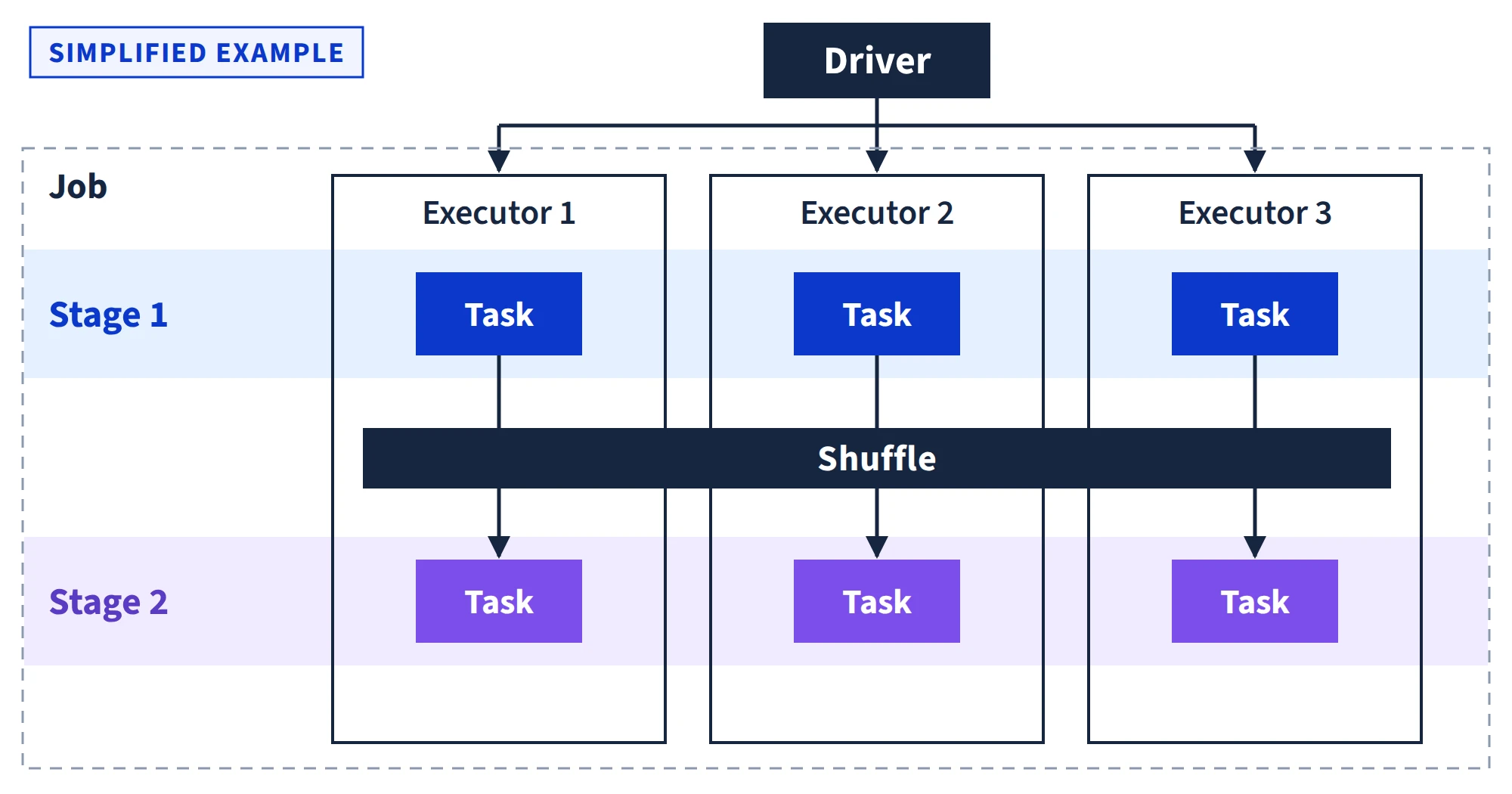
The driver runs your program. It turns your code into a plan and hands out tasks, and the executors are the worker processes that run those tasks.
Executors also keep any data you’ve cached, meaning saved in memory for reuse.
A cluster manager is the software that decides which machines the executors run on. Spark comes with its own cluster manager, and it also runs on YARN (Hadoop’s manager) and Kubernetes, a popular system for running apps.
collect() belongs in this answer too. It pulls every row back to the driver, which is a single process with limited memory. So calling it on a big table can fail the job or crash the driver (Q28).
4. What’s the Difference Between an RDD, a DataFrame, and a Dataset?
An RDD is just a collection of objects with no columns. A DataFrame has named, typed columns, so Spark can optimize it. And a Dataset is a typed DataFrame, but you only get it in Scala and Java.
A Dataset also checks those types before the code runs.
In PySpark, the choice is RDD or DataFrame, and the default answer is DataFrame. Use an RDD only for data that doesn’t fit into columns, like raw text you parse line by line.
Our tutorials on working with RDDs and working with DataFrames show both in practice.
5. What Is Lazy Evaluation in Spark?
Transformations like filter just add steps to a plan, and nothing actually runs until an action like count asks for a result. Spark waits so it can optimize the whole plan at once.
For example, Spark can combine steps and skip columns you never use. You can see lazy evaluation by timing both halves of a job. This code doubles 50 million numbers, keeps the ones divisible by 7, and counts them.
import time

start = time.time()
evens = spark.range(50_000_000).withColumn("x", F.col("id") * 2).filter("x % 7 = 0")
print(f"Transformations: {time.time() - start:.2f}s")

start = time.time()
print(evens.count())
print(f"Action: {time.time() - start:.2f}s")
Transformations: 0.18s
7142858
Action: 0.89sThe transformations came back almost instantly, because Spark hadn’t touched a row yet. All the work happened at count(). Your times will differ. The point is that the action is what starts the computation.
There’s a simple way to tell a transformation from an action. A transformation returns a new DataFrame, while an action returns a result or writes data somewhere.
6. What’s the Difference Between Narrow and Wide Transformations?
A narrow transformation, like filter, works on each partition, which is one chunk of the data, all by itself. A wide one, like groupBy, has to move rows between executors first, and that’s called a shuffle.
Each partition is processed by one task. A wide transformation, like groupBy or many joins, needs every row with the same key in one place. The key is the column you group or join on, and moving those rows between executors is the shuffle.
The shuffle is usually the most expensive part of a job. It shows up as an Exchange in the plan that explain() prints. This code prints one plan for each query. You don’t need to read every line.
# Narrow: filter and select work inside each partition
orders.filter(F.col("amount") > 50).select("customer", "amount").explain()

# Wide: groupBy has to move rows with the same key to the same place
orders.groupBy("customer").agg(F.sum("amount").alias("total")).explain()
== Physical Plan ==
*(1) Project [customer#1, amount#3]
+- *(1) Filter (isnotnull(amount#3) AND (amount#3 > 50.0))
+- *(1) Scan ExistingRDD[order_id#0,customer#1,order_date#2,amount#3]
== Physical Plan ==
AdaptiveSparkPlan isFinalPlan=false
+- HashAggregate(keys=[customer#1], functions=[sum(amount#3)])
+- Exchange hashpartitioning(customer#1, 200), ENSURE_REQUIREMENTS, [plan_id=78]
+- HashAggregate(keys=[customer#1], functions=[partial_sum(amount#3)])
+- Project [customer#1, amount#3]
+- Scan ExistingRDD[order_id#0,customer#1,order_date#2,amount#3]Scan means reading the data, Project means selecting columns, and HashAggregate is the groupBy. The numbers after # are Spark’s internal column IDs, so you can ignore them.
ExistingRDD appears because the table was built in memory from Python data rather than read from a file.
The line that matters is Exchange, and only the second plan has one. The 200 inside it is the default number of shuffle partitions.
To reduce shuffles, filter rows and drop columns before the wide step, so there’s less data to move. In a join, broadcasting a small table lets the big table skip the shuffle (Q18).
7. What Are the Catalyst Optimizer and Tungsten?
Catalyst is Spark’s query optimizer. It rewrites your code into a faster plan, and then Tungsten is the engine that runs that plan efficiently.
Tungsten stores data in a compact format and turns chains of steps into a single piece of generated code, so rows pass through without stopping between steps. You can see both at work in the filter query from Q6.
Nobody wrote isnotnull(amount), but Catalyst added it, because a missing amount can never be greater than 50. The *(1) markers show which steps Tungsten combined into one piece of code.
8. What Are Jobs, Stages, and Tasks?
Every action starts a job. Spark splits that job into stages wherever there’s a shuffle, and each stage runs one task per partition.
Spark plans a job’s steps as a DAG, short for directed acyclic graph. That’s a chain of steps that only moves forward and never loops back. A job with one groupBy usually has 2 stages, split at the shuffle.
The Spark UI is a web page that shows every job broken down this way, with the time each task took. When you run Spark locally, it’s at http://localhost:4040 by default. It’s the first place to look when something runs slow.
PySpark Coding Interview Questions
Except for Q9, which reads its own small CSV file, each coding answer runs against the orders table from Q2. So you can paste them in order and follow along.
9. How Do You Read a CSV File With a Defined Schema?
You’d pass a schema to spark.read.csv instead of turning on inferSchema. That way Spark reads the file once and uses your types instead of guessing.
With inferSchema, Spark reads the file an extra time just to guess the column types, and it can guess wrong. This code writes a small CSV file and reads it back with a schema.
import csv

with open("payments.csv", "w", newline="") as f:
    csv.writer(f).writerows([
        ["payment_id", "customer", "paid_at", "amount"],
        [1, "alice", "2026-01-03", "120.00"],
        [2, "bob", "2026-01-04", "80.50"],
    ])

payments = spark.read.csv(
    "payments.csv",
    header=True,
    schema="payment_id INT, customer STRING, paid_at DATE, amount DOUBLE",
)
payments.printSchema()
payments.show()
root
|-- payment_id: integer (nullable = true)
|-- customer: string (nullable = true)
|-- paid_at: date (nullable = true)
|-- amount: double (nullable = true)
+----------+--------+----------+------+
|payment_id|customer| paid_at|amount|
+----------+--------+----------+------+
| 1| alice|2026-01-03| 120.0|
| 2| bob|2026-01-04| 80.5|
+----------+--------+----------+------+The schema here is a DDL string, which is the same column list you’d write in a SQL CREATE TABLE. It’s the shortest way to write one. The longer form builds the same schema with StructType and StructField, which helps when your code needs to build a schema on the fly.
10. How Do You Remove Duplicate Rows?
You call dropDuplicates(), which removes rows that match on every column. If you pass it a list of columns, it keeps one row for each value of those columns.
print(orders.count(), orders.dropDuplicates().count())
print(orders.dropDuplicates(["customer"]).count())
7 6
3The table has 7 rows, 6 unique rows, and 3 customers. The second line of output shows 3 rows, one per customer. But nothing in the code said which of each customer’s rows to keep.
With a list of columns, Spark keeps whichever row it finds first, and that can change from run to run. That’s fine for a quick count. But it’s a bug if you needed the newest order. To control which row survives, use the window function in Q11.
11. How Do You Keep Only the Latest Record for Each Customer?
You number each customer’s rows from newest to oldest with row_number() over a window, and then you keep row 1.
from pyspark.sql import Window

latest_first = Window.partitionBy("customer").orderBy(F.col("order_date").desc())

(orders
    .withColumn("rn", F.row_number().over(latest_first))
    .filter("rn = 1")
    .drop("rn")
    .orderBy("customer")
    .show())
+--------+--------+----------+------+
|order_id|customer|order_date|amount|
+--------+--------+----------+------+
| 6| alice|2026-01-09| 45.0|
| 5| bob|2026-01-07| 200.0|
| 4| carol|2026-01-06| NULL|
+--------+--------+----------+------+A window function computes a value for each row from a group of related rows. Unlike groupBy, though, it keeps every row. Here, partitionBy just means “group by customer,” not the data partitions from Q6.
Sorting the text column order_date works because the dates are written year first. Bob’s 2 identical orders tie, so either one is correct.
Ties are where the 3 numbering functions differ. Suppose you rank scores from highest to lowest, 2 rows tie at 10, and a third has 5. Then row_number gives 1, 2, 3, rank gives 1, 1, 3, and dense_rank gives 1, 1, 2.
Use row_number when you need exactly one row per position, rank when ties should share a rank and leave gaps, and dense_rank when ties should share a rank without gaps.
12. How Do You Calculate a Running Total per Customer?
You use sum() over a window that’s grouped by customer and sorted by date. The frame, meaning the rows the sum covers, runs from the first row up to the current one.
from pyspark.sql import Window

running = (Window.partitionBy("customer")
           .orderBy("order_date")
           .rowsBetween(Window.unboundedPreceding, Window.currentRow))

(orders.dropDuplicates()
    .withColumn("running_total", F.sum("amount").over(running))
    .orderBy("customer", "order_date")
    .show())
+--------+--------+----------+------+-------------+
|order_id|customer|order_date|amount|running_total|
+--------+--------+----------+------+-------------+
| 1| alice|2026-01-03| 120.0| 120.0|
| 3| alice|2026-01-05| 60.0| 180.0|
| 6| alice|2026-01-09| 45.0| 225.0|
| 2| bob|2026-01-03| 80.0| 80.0|
| 5| bob|2026-01-07| 200.0| 280.0|
| 4| carol|2026-01-06| NULL| NULL|
+--------+--------+----------+------+-------------+The code drops duplicates first, so Bob’s repeated order counts once and his total is 280, not 480. Carol’s running total is NULL, because her only amount is NULL. Duplicates and missing values are the 2 things to check in any running total.
13. How Do You Handle Missing Values?
First you count how many are missing. Then you decide whether to drop them, fill them, or leave them, and that depends on what the numbers are for.
dropna drops rows and fillna fills in a value. Dropping loses rows, and filling changes totals and averages.
count("*") counts every row, while count("amount") skips nulls. So the difference between the 2 is your null count.
orders.select(
    F.count("*").alias("rows"),
    F.count("amount").alias("amount_not_null"),
    F.avg("amount").alias("avg_amount"),
).show()

orders.fillna({"amount": 0.0}).filter("customer = 'carol'").show()
+----+---------------+----------+
|rows|amount_not_null|avg_amount|
+----+---------------+----------+
| 7| 6| 117.5|
+----+---------------+----------+
+--------+--------+----------+------+
|order_id|customer|order_date|amount|
+--------+--------+----------+------+
| 4| carol|2026-01-06| 0.0|
+--------+--------+----------+------+The average of 117.5 ignored Carol’s missing amount. The 6 real amounts, including Bob’s duplicate, add up to 705. If you filled Carol’s with 0 first, you’d divide 705 by 7 instead of 6, and the average would drop to about 100.7.
14. What Join Types Does PySpark Support?
You’ve got inner, left, right, full outer, and cross joins, plus left_semi and left_anti.
A left_semi join keeps the left rows that have a match, and left_anti keeps the ones that don’t. Neither adds any columns from the right table.
customers = spark.createDataFrame(
    [("alice", "US"), ("bob", "UK"), ("carol", "DE"), ("dev", "IN")],
    "customer STRING, country STRING",
)

# Customers who have never ordered
customers.join(orders, "customer", "left_anti").show()
+--------+-------+
|customer|country|
+--------+-------+
| dev| IN|
+--------+-------+Dev is the only customer with no orders, so left_anti returns just that row. You pick the join type with the third argument, as in orders.join(customers, "customer", "left"). With no third argument, the join is inner.
Be careful with a cross join. It pairs every row of one table with every row of the other, so 1,000 rows times 1,000 rows gives you a million.
15. When Should You Use a UDF, and What Does It Cost?
You’d only use a UDF, a user-defined function, when no built-in function can do the job. They’re slower, and Spark can’t optimize what happens inside them.
Spark itself runs on the JVM, the Java runtime. Your UDF is Python code, which the JVM can’t run. So every value has to be sent from Java to a separate Python process and back.
from pyspark.sql.functions import udf

shout = udf(lambda s: s.upper() if s else None, "string")

orders.select(shout("customer").alias("c")).explain()
orders.select(F.upper("customer").alias("c")).explain()
== Physical Plan ==
*(2) Project [pythonUDF0#171 AS c#170]
+- ArrowEvalPython [<lambda>(customer#1)#169], [pythonUDF0#171], 101
+- *(1) Project [customer#1]
+- *(1) Scan ExistingRDD[order_id#0,customer#1,order_date#2,amount#3]
== Physical Plan ==
*(1) Project [upper(customer#1) AS c#172]
+- *(1) Scan ExistingRDD[order_id#0,customer#1,order_date#2,amount#3]The UDF plan adds an ArrowEvalPython step, while the built-in upper() stays inside one piece of generated code.
Spark 4.2 made regular UDFs faster (Q24). But a pandas UDF can be faster still, because your function runs once per batch on a whole pandas Series, instead of once per value.
PySpark Performance and Optimization Questions
The coding questions show you can write PySpark. The next questions test whether you can make it run fast.
To see these fixes applied to a real slow pipeline, try our PySpark performance tuning tutorial.
16. What’s the Difference Between repartition and coalesce?
repartition(n) shuffles the data into n roughly even partitions, so it can go up or down. coalesce(n) merges the partitions you already have without a shuffle, so it’s cheaper, but it can only go down.
Here’s each one asked for a specific number of partitions.
nums = spark.range(1_000_000, numPartitions=4)
print(nums.rdd.getNumPartitions())
print(nums.repartition(8).rdd.getNumPartitions())
print(nums.coalesce(2).rdd.getNumPartitions())
print(nums.coalesce(64).rdd.getNumPartitions())
4
8
2
4The code sets 4 partitions up front, so you’ll see the same output on any machine. repartition(8) shuffled the rows into 8, and coalesce(2) merged them down to 2 without a shuffle.
But coalesce(64) stayed at 4, because merging can’t create partitions, and Spark didn’t raise an error.
coalesce(1) has a different risk. Because it doesn’t add a shuffle, it can pull the steps before it into a single task too.
If you need one output file, repartition(1) adds a shuffle but keeps that earlier work running in parallel.
17. How Many Partitions Should a Job Have?
It depends on your data and your cluster. You’d want enough partitions to keep every CPU core busy, but not so many that each one is tiny and the overhead takes over.
The Spark tuning guide suggests 2 to 3 tasks per CPU core. Too few partitions leave cores sitting idle. Too many add overhead for every task Spark has to schedule, and they write lots of tiny files.
When Spark reads files, it splits them into chunks of up to 128 MB. After a shuffle, you start with 200 partitions by default. Then Adaptive Query Execution (AQE) adjusts them while the job runs, using the actual data sizes.
AQE merges small shuffle partitions based on the data it actually sees. By default, it favors keeping every core busy over hitting any fixed size. It can merge partitions but not split them, except in skewed joins (Q19).
In practice, start with Spark’s defaults and let AQE adjust. Tune when the Spark UI shows idle cores, tasks so big they spill to disk, or lots of tiny tasks. For a very large shuffle, that can mean raising spark.sql.shuffle.partitions.
18. What Is a Broadcast Join, and When Should You Use One?
A broadcast join sends a full copy of the small table to every executor, so the big table doesn’t have to shuffle. You’d use it when one side of the join is small enough to fit in each executor’s memory.
Spark broadcasts a table on its own when it estimates the table is under 10 MB, but it needs usable size statistics to do that. The customers table is tiny, so it’s a good broadcast candidate.
But Spark doesn’t know the size of a table built from Python data, so in our test this join ran as a sort-merge join (Q26) without a hint.
That’s why the code forces the broadcast with broadcast().
orders.join(F.broadcast(customers), "customer").explain()== Physical Plan ==
AdaptiveSparkPlan isFinalPlan=false
+- Project [customer#1, order_id#0, order_date#2, amount#3, country#161]
+- BroadcastHashJoin [customer#1], [customer#160], Inner, BuildRight, false, false
:- Filter isnotnull(customer#1)
: +- Scan ExistingRDD[order_id#0,customer#1,order_date#2,amount#3]
+- BroadcastExchange HashedRelationBroadcastMode(List(input[0, string, false]),false), [plan_id=765]
+- Filter isnotnull(customer#160)
+- Scan ExistingRDD[customer#160,country#161]Most of this output is Spark bookkeeping. The line to look for is BroadcastHashJoin, which confirms it worked. BroadcastExchange is the small table being copied out, not a shuffle.
Broadcasting a table that’s too big can run the driver or the executors out of memory, because the driver collects the whole table before sending it out. If that happens, you can turn automatic broadcasts off with spark.conf.set("spark.sql.autoBroadcastJoinThreshold", -1).
19. What Is Data Skew, and How Do You Fix It?
Skew is when a few keys, called hot keys, hold most of the rows, so one task runs way longer than the rest. You can fix it by broadcasting, letting AQE split skewed joins, or salting the hot key.
The right fix depends on where the skew shows up.
- Broadcast the smaller table. This works when the skew is in a join, because the big table never shuffles.
- Let AQE split skewed joins. AQE has been on by default since Spark 3.2, but it only handles skew in sort-merge joins, not in
groupByaggregations. Check the stage in the Spark UI to see whether it already evened out the task times. - Salt the hot key. This is the fix for a skewed aggregation. Add a random number to the end of the key, so its rows spread across several partitions. Then aggregate twice, first by the salted key and then by the original key.
20. What’s the Difference Between cache and persist?
They both keep a computed DataFrame around, so later actions don’t have to recompute it. cache() uses the default storage level, and persist() lets you pick one.
The default uses both memory and disk. This code caches one DataFrame and persists another to disk only.
from pyspark import StorageLevel

cached = orders.cache()
cached.count()
print(cached.storageLevel)

on_disk = orders.dropDuplicates().persist(StorageLevel.DISK_ONLY)
on_disk.count()
print(on_disk.storageLevel)
Disk Memory Deserialized 1x Replicated
Disk Serialized 1x ReplicatedIn the first output line, Disk Memory means Spark keeps the data in memory and spills to disk when memory runs out.
Notice the count() after each call. cache() is lazy, just like a transformation, so nothing is stored until the next action runs. Cache only what you reuse, and call unpersist() when you’re done with it.
21. What Is Predicate Pushdown, and Why Does Parquet Help?
Predicate pushdown means Spark applies a filter condition, like amount > 50, while it’s reading the data instead of after. Parquet helps because it lets Spark skip data that can’t match.
Parquet stores data by column and keeps the smallest and largest value for each block of rows. So Spark can skip blocks that can’t match, and read only the columns you asked for.
CSV and JSON files don’t keep those per-block values, so Spark has to read every row.
You can also save files into folders by a column like date, which is a third use of the word “partition,” after data partitions (Q6) and window groups (Q11). Then a filter on that column skips whole folders, which is called partition pruning.
PySpark Questions That Changed in Spark 4
Spark 4.0 came out in May 2025, and 4.2.0 followed in July 2026. The answers in this section changed with those releases.
This table shows which version changed each default. Check the last column against anything you’re studying.
| Setting or behavior | Before | Now | Since |
|---|---|---|---|
spark.sql.adaptive.enabled (AQE) | Off | On | 3.2 |
spark.sql.ansi.enabled (strict casts and math) | Off | On | 4.0 |
spark.sql.execution.pythonUDF.arrow.enabled | Off | On | 4.2 |
spark.sql.execution.arrow.pyspark.enabled (Arrow for toPandas()) | Off | On | 4.2 |
| Minimum Python version | 3.9 | 3.10 | 4.1 |
22. What Happens When a Value Can’t Be Cast to the Target Type?
Since Spark 4.0, if you cast a value to a type it can’t become, like the text “n/a” to a number, the job fails with a CAST_INVALID_INPUT error. Before 4.0, you’d quietly get a NULL.
The change happened because ANSI mode is on by default now, which makes Spark follow the SQL standard’s stricter rules.
This code tries to convert the text “n/a” to an integer, first the plain way and then with try_cast. It trims the long error message down to its first line.
raw = spark.createDataFrame([("42",), ("n/a",)], "amount STRING")

try:
    raw.select(F.col("amount").cast("int")).show()
except Exception as e:
    print(type(e).__name__)
    print(str(e).split(". Correct")[0])

raw.select(F.expr("try_cast(amount AS INT)").alias("amount")).show()
NumberFormatException
[CAST_INVALID_INPUT] The value 'n/a' of the type "STRING" cannot be cast to "INT" because it is malformed
+------+
|amount|
+------+
| 42|
| NULL|
+------+When you run this yourself, your console also prints a long Java error log. That’s expected, so you can scroll past it.
The plain cast stopped the whole query. The first output line is the error’s type, and the second is Spark’s message, which names the value that broke it. (PySpark names the error after the Java exception underneath it.)
try_cast brings back the old NULL behavior, on purpose this time. Division by zero changed the same way. It now raises DIVIDE_BY_ZERO unless you use try_divide.
23. What Is Spark Connect?
Spark Connect splits PySpark into a small client and a remote Spark server. Your code sends DataFrame plans to the server, and the server does the heavy lifting.
Spark Connect doesn’t support the RDD API or SparkContext, so you give up both. You often can’t tell whether a team uses it, so DataFrame-only answers are the safe default.
To connect, you call SparkSession.builder.remote() with a server address, and most DataFrame code runs unchanged.
24. Are Python UDFs Still Slow in Spark 4?
They’re still slower than built-in functions, but they’re faster than they used to be. That’s because Spark 4.2 moves their data in batches with Arrow by default.
Arrow is a column-based format for moving data between Java and Python, and it’s the ArrowEvalPython step you saw in Q15. Arrow speeds up moving the data. But your function still runs once per value. The PySpark 4.2 upgrade notes list the change.
This only works when pandas and PyArrow are installed. Without them, Spark falls back to the older, slower path and prints a warning. The install command in Q2 includes both.
Scenario-Based PySpark Interview Questions for Experienced Candidates
Scenario questions don’t have one right answer. The interviewer wants to hear how you’d work through the problem, step by step.
25. A Job That Took 10 Minutes Now Takes 2 Hours. What Do You Do?
You diagnose before you tune. You find the slowest stage in the Spark UI, figure out why it’s slow, fix that, and then confirm the fix worked.
In the slowest stage, check for one task running far longer than the rest (skew), data spilling to disk because it doesn’t fit in memory (partitions too big), or simply more input than before.
Next, check what changed recently, like data volume, a new join, or a config change. Once you’ve picked a fix, rerun the job and compare the same stage in the Spark UI, to confirm the fix worked.
Adding more executors is the tempting first move. But if one skewed task is the problem, more executors just cost more money, because that task still runs alone.
26. How Would You Join Two Very Large Tables?
You shrink both tables before the join, and then you check the join keys for skew.
Neither table is small enough to broadcast, so both will shuffle. Filter the rows and select only the columns you need before joining.
Without a broadcast, Spark usually picks a sort-merge join for a join on matching keys. It can also choose a shuffled hash join, and AQE can switch strategies while the job runs, based on the actual data sizes.
A sort-merge join shuffles both tables by the join key, sorts them, and then walks through them side by side.
If your team joins the same 2 tables often, you can save them bucketed, meaning pre-split by the join key. When both tables use the same key and the same number of buckets, later joins can skip the shuffle.
27. How Do You Avoid Writing Thousands of Tiny Files?
You cut the number of partitions before you write, because each task writes at least one file.
With 200 shuffle partitions, that can mean 200 files. And if you split the output into folders by date, each folder can get 200 files, because any task can hold rows for any date.
Use coalesce to lower the number of partitions before writing, or repartition on the column you split the folders by, so each folder gets one file. AQE’s partition merging helps too.
Tiny files mostly hurt the jobs that read them later. Every file has to be opened and scheduled, so thousands of small files read far slower than a few large ones.
28. How Do You Troubleshoot Out-of-Memory Errors?
The first thing you figure out is whether it was the driver or an executor that ran out of memory, because the causes are different.
A driver out-of-memory error (OOM) usually means too much data came back to it, often from collect() or toPandas(). Spark has a guard for this. By default, it stops any action whose results add up to more than 1 GB on the way back to the driver.
That limit doesn’t make the driver safe, though. Rows take up more memory once they’re unpacked, so a driver can still run out below 1 GB. The better fix is to bring back less data.
An executor OOM usually points to skew or oversized partitions. More memory only raises the limit, and the next bigger hot key breaks it again. So spreading the data out with more partitions or a skew fix works better.
Quick-Fire PySpark Interview Questions
A one- or two-sentence answer is usually enough for these.
29. How Is Spark Different From Hadoop MapReduce?
Spark plans the whole job as one graph and runs chains of steps together. MapReduce, Hadoop’s older batch engine, writes results to disk after every map and reduce step. Spark can also cache data you reuse, so it’s usually much faster for jobs with many steps.
Spark still writes shuffle data to disk, so “memory versus disk” oversimplifies it. The real gain is that Spark skips the disk writes between steps that don’t need a shuffle.
30. What’s the Difference Between map and flatMap?
map gives you exactly one output for each input. flatMap can give you zero or more and flattens them into one list.
Both are RDD methods. Say your 2 input strings are “a b” and “c”, and you split each on spaces. map gives [['a', 'b'], ['c']], and flatMap gives ['a', 'b', 'c'].
On a DataFrame, you’d get the same result with split(), which makes a list, followed by explode(), which turns each list item into its own row.
31. What’s the Difference Between reduceByKey and groupByKey?
reduceByKey combines values inside each partition before the shuffle, so it moves a lot less data than groupByKey.
Both group key-value pairs in an RDD. groupByKey sends every single value across the network.
With DataFrames, you don’t have to choose. groupBy().agg() already combines values before the shuffle, and that’s the partial_sum step in the plan from Q6.
32. What Are Accumulators?
Accumulators are counters that executors add to and only the driver can read. You’d use one for something like counting bad records.
Only trust the count when you update it inside an action, like foreach(). If you update it inside a transformation, a task that fails and reruns adds its count twice, so the total can come out too high.
33. What Are Broadcast Variables?
A broadcast variable is a read-only value, like a lookup dictionary, that Spark sends to each executor once instead of with every task.
You create one with spark.sparkContext.broadcast(), so it isn’t available on Spark Connect.
Broadcast variables use the same idea as the broadcast join in Q18, but for a plain Python value. Without one, a large dictionary used inside a UDF gets sent again with every task.
34. How Does Spark Recover From a Failed Task?
Spark remembers the steps that built each partition, which is called its lineage. If a partition gets lost, Spark reruns those steps.
That way, it doesn’t need to keep extra copies of the data. Lineage works because DataFrames are immutable, meaning they never change after they’re created. Every step makes a new DataFrame instead of editing the old one, so the steps to rebuild a partition always still apply.
35. What Does checkpoint() Do?
checkpoint() saves a DataFrame to storage and cuts its lineage, so Spark doesn’t have to rebuild it from scratch.
That helps when the list of steps gets very long, for example in a loop that adds steps on every pass. Unlike cache() from Q20, a checkpoint is written to shared storage like HDFS or Amazon S3, so it survives a lost executor.
Writing to shared storage makes a checkpoint slower than caching. You also have to set a checkpoint folder first, with spark.sparkContext.setCheckpointDir().
36. What Is spark-submit?
spark-submit is the command you use to launch a Spark application on a cluster.
It’s where you set things like executor memory, the number of executors, and which cluster manager to use. It also sets the deploy mode, which decides where the driver runs.
In client mode, the driver runs on the machine where you launched the job. In cluster mode, it runs inside the cluster. That suits scheduled production jobs, because the job keeps running even if the machine that launched it disconnects.
37. What Is Structured Streaming?
Structured Streaming handles data that keeps arriving, and it uses the same DataFrame API as your batch jobs.
By default, it works in small batches. It also saves its progress to a checkpoint folder, so a restarted query picks up where it left off. That’s a different feature from checkpoint() in Q35.
You write the query like a batch query, and Spark keeps running it as new data arrives. The output mode decides what each batch writes.
- Append writes only new rows.
- Complete rewrites the whole result.
- Update writes only the rows that changed.
38. What Is Executor Memory Overhead?
It’s extra memory each executor gets outside the JVM’s own memory, and PySpark’s Python processes use it. By default it’s 10% of executor memory, or 40% for non-JVM jobs like PySpark on Kubernetes, with a 384 MB minimum.
If YARN or Kubernetes kills a PySpark executor for using too much memory, the Python processes may be what ran out. So raise the overhead rather than the executor memory. Jobs with heavy Python UDFs hit this more often than pure DataFrame jobs.
39. How Does Spark Serialize Data?
Spark turns objects into bytes so it can send or store them. The default is Java serialization, and Kryo is the faster option.
This conversion is called serializing. Kryo is more compact too, and it matters most for jobs that use RDDs heavily.
For DataFrames the choice matters less, because Tungsten (Q7) already stores rows in its own compact format. If you do want Kryo, you switch to it with the spark.serializer setting.
40. What Is Speculative Execution?
Speculative execution runs a backup copy of a slow task on another executor and keeps whichever one finishes first. It’s off by default.
Speculation helps when a few slow machines drag out a stage. But it doesn’t help with skew (Q19). A skewed task is slow because it has more data, and a backup copy has the same data.
41. How Do You Read Data From a Relational Database?
You use spark.read.jdbc() with the database URL and table name. If you add a partition column with bounds, Spark can read the table in parallel.
JDBC is Java’s standard way to connect to databases like PostgreSQL or MySQL.
The arguments are column, lowerBound, upperBound, and numPartitions. The column has to hold numbers, dates, or timestamps. If you use spark.read.format("jdbc") instead, these become options, and the column one is called partitionColumn.
The bounds only decide how Spark splits the reads, and they don’t filter out any rows. Without these arguments, a single task reads the whole table over one connection, no matter how big your cluster is.
42. How Do You Count Distinct Values in a Column?
You’d use countDistinct() for an exact count, or approx_count_distinct() when the data is huge and an estimate is good enough.
orders.select("customer").distinct().count() works too. Both exact methods shuffle every distinct value across the network.
approx_count_distinct() uses an algorithm called HyperLogLog instead. It estimates the count from a small summary of each partition, so it trades a small error for far less memory and data movement.
How to Prepare for a PySpark Interview
What to Do This Week
- Install PySpark 4.2 locally and run the setup code in Q2. Then run each coding example and change one thing to see what breaks.
- Run
explain()on 3 queries of your own, including at least onegroupBy. Find theExchangein each wide query and explain why it’s there. If you only practice one skill, make it this one, because most performance answers start with reading a plan like this. - Write Q11 and Q12 from memory. Keeping the latest row and the running total are 2 window patterns to know by heart.
- Cast a text column with a bad value to a number. ANSI mode is already on in Spark 4, so you’ll see the error. Then fix it with
try_cast. - Talk through Q25 in under 2 minutes, without notes. Cover how you’d find the cause, fix it, and confirm the fix worked.
Fluency takes longer than a few weeks of prep. Databricks, the company founded by Spark’s creators, recommends 6 months or more of hands-on Spark work before its $200 associate developer exam.
The Databricks certificate can help your resume get through the first screening. But the technical interview still tests what you can do.
If your interview also has SQL questions, practice with our SQL interview questions. For more Python practice, try our Python interview questions, and for data engineering questions, see our data engineering interview questions guide.
For structured practice, Dataquest’s Distributed Data Processing with PySpark skill path includes Analyzing Large Datasets in Spark and PySpark for Data Engineering.
The PySpark courses cover pipelines, performance tuning, and running PySpark in the cloud. You write code in the browser and get feedback as you go.
Both courses are also part of the full Data Engineer path.
FAQ
How hard is PySpark if you already know pandas?
The DataFrame idea will feel familiar right away. The harder part is thinking about partitions, shuffles, and lazy evaluation, because pandas never makes you do that.
Are Databricks PySpark interviews different?
The PySpark questions are the same, since Databricks runs Apache Spark. But expect extra questions on the platform itself, like Delta Lake, its table format, and how jobs get scheduled there.
Is PySpark or Scala better for Spark jobs?
Both show up about equally. In InterviewStack’s May 2026 analysis, 13% of data engineer postings named PySpark and 12% named Scala. The DataFrame API works the same way in both languages, so the concepts carry over if you switch later.
How do you practice without a cluster?
Run Spark on your own laptop in local mode. The install steps in Q2 are all you need for every example in this post.
Our PySpark tutorial for beginners walks through the setup in more detail. Use Java 17 or 21 even if it shows an older version.
