Window Functions in SQL
Have you ever felt like you're only scratching the surface of what SQL can do? SQL, a powerful tool for managing and analyzing data, has advanced features that many users overlook. One such feature is window functions. Let me explain why.
Window functions allow you to perform calculations across a set of rows related to the current row, all while keeping the detail of your data intact. It's like having the best of both worlds – you get to maintain the granularity of your data while still performing complex calculations.
When I first started learning window functions, I realized that I could use them in some of the course performance reports I run regularly. If we wanted to, we could use them daily to gain insights into student progress and course effectiveness. For example, we could easily calculate the moving average of course completions over time, giving us a clear picture of engagement trends. But instead, the SQL scripts I use contain subqueries and self-joins, which I discussed in previous posts. This is totally fine, and the results are accurate, but the code and logic is often more complex than if we used window functions.
Window functions simplify queries. I used to struggle with complicated subqueries and self-joins, but window functions often replace them with cleaner, more efficient code. This makes our queries easier to write and maintain, and it also significantly improves performance, especially when we're dealing with large datasets.
There's a whole range of window functions, each with its own unique capabilities. We have aggregate functions like SUM and AVG that you might already know, but used as window functions. Then there are ranking functions like ROW_NUMBER and RANK, which we use for everything from simple numbering to complex sales analysis. Distribution functions like PERCENT_RANK are great for statistical analysis, and offset functions like LAG and LEAD help us identify trends.
In this post, we'll explore these different types of window functions and see how they can enhance your approach to data analysis. We'll start with the basics of syntax and concepts, then move on to more advanced applications. Whether you're just starting out with SQL or looking to improve your skills, understanding window functions can open up exciting new possibilities in your data analysis toolkit.
Let's begin our exploration with an introduction to window functions and how they work. Trust me, once you get the hang of these, you'll wonder how you ever managed without them!
Lesson 1 – An Introduction to Window Functions

Imagine being able to analyze your data in a way that reveals hidden trends and patterns. That's exactly what window functions can do. Recall that window functions allow you to perform calculations across a set of related rows while keeping all your original data intact.
So, how do window functions work? The key is the OVER clause, which defines the "window" of rows the function will operate on. Let's take a look at an example:
SELECT bike_number, member_type, duration,
       AVG(duration) OVER (PARTITION BY member_type) AS avg_trip_duration
  FROM tbl_bikeshare;
In this query, we're calculating the average trip duration for each member type. The PARTITION BY member_type part of the OVER clause tells SQL to create separate windows for each member type.
Here's what the output might look like:
| bike_number | member_type | duration | avg_trip_duration |
|---|---|---|---|
| W20796 | Casual | 3151 | 2223.74 |
| W01168 | Casual | 2810 | 2223.74 |
| W23045 | Casual | 648 | 2223.74 |
| W21185 | Casual | 997 | 2223.74 |
| W00900 | Casual | 1821 | 2223.74 |
| W22778 | Casual | 885 | 2223.74 |
| ... | ... | ... | ... |
You can see how each row shows both the individual trip duration and the average for that member type. That's the beauty of window functions – you get to keep all your detailed data while also seeing the big picture.
You might be wondering, "Couldn't I just use GROUP BY for this?" Well, let's compare:
SELECT member_type,
       AVG(duration) AS avg_trip_duration
  FROM tbl_bikeshare
 GROUP BY member_type;
This gives us:
| member_type | avg_trip_duration |
|---|---|
| Casual | 2223.74 |
| Member | 733.07 |
While we get the average trip durations, we've lost all the individual trip data. With window functions, we keep both.
As you continue with learning SQL, you'll find that window functions open up a world of possibilities for data analysis. They allow you to perform complex calculations and comparisons without losing the details of your data. Whether you're analyzing bike share data, student performance, or any other dataset, window functions can help you uncover insights you might otherwise miss.
By learning window functions, you'll be able to gain a deeper understanding of your data and make more informed decisions. So, take the time to experiment and see what insights you can uncover. You might just find that window functions become your go-to tool for data analysis.
Lesson 2 – Window Function Framing

When I first learned about window functions, I realized I had discovered a powerful tool for data analysis. But then I checked out window function framing, and I gained a new level of precision in my data analysis. I'd like to share this insight with you.
Window framing allows you to define a specific set of rows within your partition to perform calculations on. Think of it as a magnifying glass that lets you focus on particular sections of your data. This approach is particularly valuable when analyzing time-series data or calculating rolling totals.
To define a window frame, you'll use the ROWS or RANGE keywords, along with frame bounds like PRECEDING, FOLLOWING, and CURRENT ROW. Here's an example of how to calculate a running total of product sales:
SELECT *,
       SUM(quantity) OVER (
              ORDER BY sales_date
              ROWS BETWEEN UNBOUNDED PRECEDING AND CURRENT ROW
           ) AS running_total_quantity
  FROM apple_sales_quantity_by_month;
This query gives us:
| sales_date | brand | quantity | running_total_quantity |
|---|---|---|---|
| 2022-01-31 | Apple | 50 | 50 |
| 2022-02-28 | Apple | 40 | 90 |
| 2022-03-31 | Apple | 25 | 115 |
| 2022-04-30 | Apple | 30 | 145 |
| 2022-05-31 | Apple | 47 | 192 |
| 2022-06-30 | Apple | 40 | 232 |
Lesson 3 – Window Aggregate Functions
As the animation above shows, when you write aggregate queries, the columns not included in the GROUP BY clause do not appear in the result set, and you lose the details. Window aggregate functions empower you to perform calculations across rows while preserving your original data intact, giving you a more comprehensive understanding of your data.
Let me explain how they work. Window aggregate functions utilize an OVER clause, which defines the set of rows we're working with – our 'window' of data. Here's a simple example:
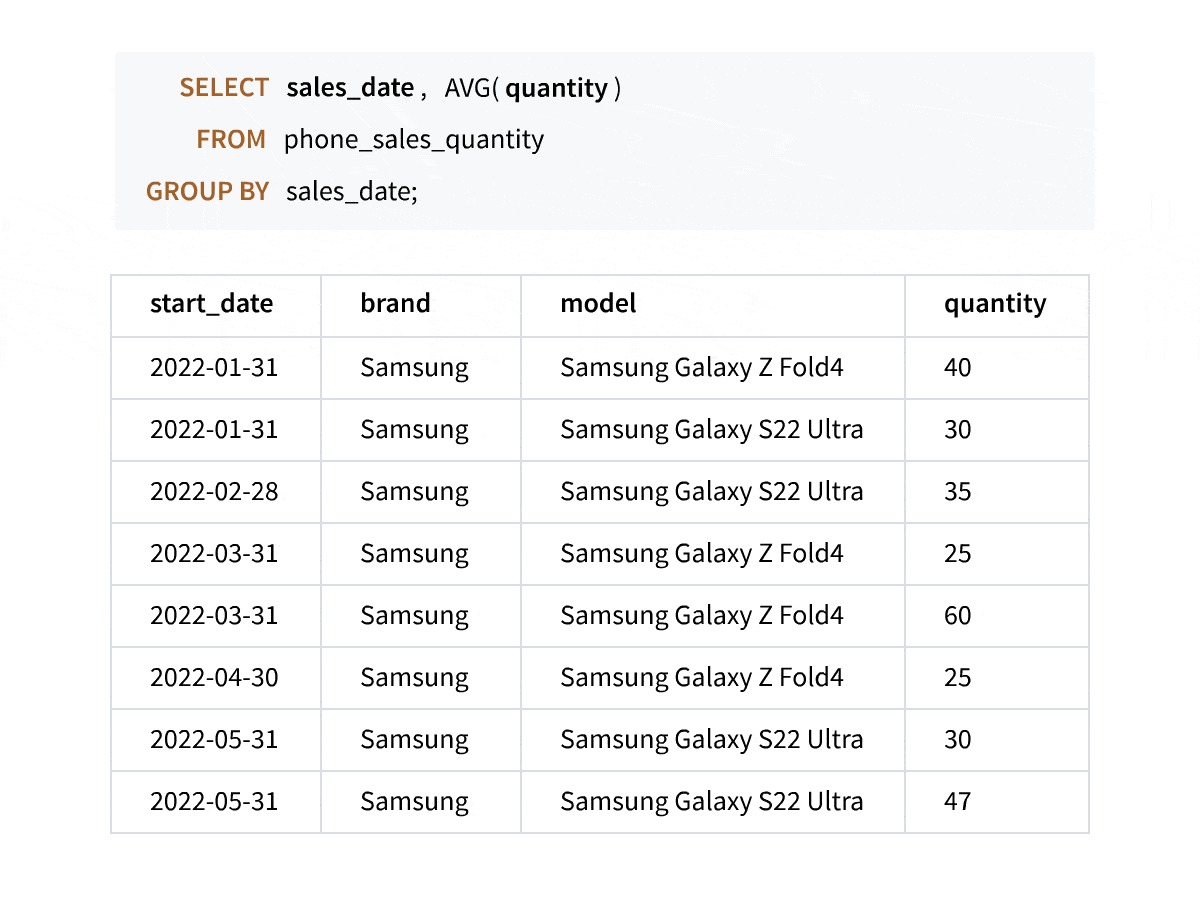
SELECT sales_date, brand, model, quantity,
       SUM(quantity) OVER (PARTITION BY sales_date),
       AVG(quantity) OVER (PARTITION BY sales_date)
  FROM phone_sales_quantity;
In this query, we're calculating the sum and average quantity of phones sold each day. The PARTITION BY part tells SQL to create separate windows for each sales date, allowing us to see both aggregate calculations and individual sales data. Check it out:
| sales_date | brand | model | quantity | sum | avg |
|---|---|---|---|---|---|
| 2022-01-31 | Samsung | Samsung Galaxy Z Fold4 | 40 | 70 | 35 |
| 2022-01-31 | Samsung | Samsung Galaxy S22 Ultra | 30 | 70 | 35 |
| 2022-02-28 | Samsung | Samsung Galaxy S22 Ultra | 35 | 35 | 35 |
| 2022-03-31 | Samsung | Samsung Galaxy S22 Ultra | 25 | 85 | 42.5 |
| 2022-03-31 | Samsung | Samsung Galaxy Z Fold4 | 60 | 85 | 42.5 |
| 2022-04-30 | Samsung | Samsung Galaxy Z Fold4 | 25 | 25 | 25 |
| 2022-05-31 | Samsung | Samsung Galaxy Z Fold4 | 30 | 77 | 38.5 |
| 2022-05-31 | Samsung | Samsung Galaxy S22 Ultra | 47 | 77 | 38.5 |
| 2022-06-30 | Samsung | Samsung Galaxy Z Fold4 | 76 | 76 | 76 |
But it gets even more powerful. We can refine our windows using a window frame. Check this out:
SELECT *,
       AVG(quantity * unit_price) OVER (
              PARTITION BY brand
              ORDER BY sales_date
              ROWS BETWEEN UNBOUNDED PRECEDING AND CURRENT ROW
           ) AS running_average,
       AVG(quantity * unit_price) OVER (
              PARTITION BY brand
              ORDER BY sales_date
              ROWS BETWEEN 2 PRECEDING AND CURRENT ROW
           ) AS three_month_average
  FROM phone_sales_by_month;
This query performs two different calculations. The first, 'running_average', calculates the average sales from the start of our data up to each row. The second, 'three_month_average', uses just the current row and the two preceding it. This is particularly useful for tracking trends over time. Like this:
| sales_date | brand | model | quantity | unit_price | running_average |
|---|---|---|---|---|---|
| 2022-01-31 | Apple | iPhone 13 Pro | 50 | 999 | 49950 |
| 2022-02-28 | Apple | iPhone 13 Pro | 40 | 999 | 44955 |
| 2022-03-31 | Apple | iPhone 13 Pro | 38 | 999 | 42624 |
| ... | ... | ... | ... | ... | ... |
When using window aggregate functions, keep the following in mind:
- Be thoughtful about your
PARTITION BYclause. It should group your data in a way that makes sense for what you're trying to analyze. - Keep an eye on performance. These functions can be slower with extremely large datasets.
- Remember that window functions are calculated after most other parts of the query, including the
WHEREandORDER BYclauses. This can affect how you structure complex queries.
Window aggregate functions enable me to ask more complex questions and obtain more nuanced answers, all without losing the details in my dataset. As you continue learning SQL, you'll likely find more ways to leverage these powerful tools to gain deeper insights into your data.
Next, let's explore ranking window functions.
Lesson 4 – Ranking Window Functions

When I first used ranking functions, I could easily identify top performers, group data logically, and reveal trends that might otherwise go unnoticed. Let's explore how these functions work and how you can use them in your own projects.
We'll start with the ROW_NUMBER() function. This function assigns a unique number to each row in your result set. Here's an example using our bike-sharing data:
SELECT start_date, bike_number, member_type, rider_rating,
       ROW_NUMBER() OVER (ORDER BY rider_rating DESC) AS row_num
  FROM trips;
This query assigns a row number to each trip, ordered by rider rating from highest to lowest. I often use this when I need to identify the top N results or create unique identifiers for each row. For instance, you could use it to find the top 10 highest-rated trips of the month. Here's a snippet of the results:
| start_date | bike_number | member_type | rider_rating | row_num |
|---|---|---|---|---|
| 2017-10-04 08:30:00 | W22517 | Casual | 5 | 1 |
| 2017-10-04 04:58:00 | W23052 | Casual | 5 | 2 |
| 2017-10-03 12:00:00 | W22965 | Casual | 5 | 3 |
| 2017-10-05 08:08:00 | W00895 | Casual | 4 | 4 |
| 2017-10-02 03:30:00 | W21096 | Member | 4 | 5 |
| ... | ... | ... | ... | ... |
Next, let's look at the RANK() and DENSE_RANK() functions. These are similar to ROW_NUMBER(), but they handle ties differently. RANK() leaves gaps in the ranking when there are ties, while DENSE_RANK() doesn't. Here's an example that compares all three:
SELECT start_date, bike_number, member_type, rider_rating,
       ROW_NUMBER() OVER (ORDER BY rider_rating DESC),
       RANK() OVER (ORDER BY rider_rating DESC),
       DENSE_RANK() OVER (ORDER BY rider_rating DESC)
  FROM trips;
This query gives us:
| start_date | bike_number | member_type | rider_rating | row_number | rank | dense_rank |
|---|---|---|---|---|---|---|
| 2017-10-04 08:30:00 | W22517 | Casual | 5 | 1 | 1 | 1 |
| 2017-10-04 04:58:00 | W23052 | Casual | 5 | 2 | 1 | 1 |
| 2017-10-03 12:00:00 | W22965 | Casual | 5 | 3 | 1 | 1 |
| 2017-10-05 08:08:00 | W00895 | Casual | 4 | 4 | 4 | 2 |
| 2017-10-02 03:30:00 | W21096 | Member | 4 | 5 | 4 | 2 |
| ... | ... | ... | ... | ... | ... | ... |
Notice how RANK() jumps from 1 to 4, while DENSE_RANK() goes from 1 to 2. This difference can be crucial depending on your analysis needs. For example, if you're ranking sales performance and want to highlight the top 3 salespeople, RANK() would ensure you're not giving out more than three "medals" even if there are ties.
Lastly, let's explore the NTILE() function. This function is great for dividing your data into a specified number of groups. Here's an example:
SELECT start_date, bike_number, rider_rating,
       NTILE(2) OVER (
              PARTITION BY EXTRACT(DAY FROM start_date)
              ORDER BY rider_rating DESC
           )
  FROM trips;
This query divides each day's trips into two groups based on rider ratings. It's particularly useful for creating percentiles or segmenting data for analysis. You could use this to identify the top 50% of rated trips each day, which might be valuable for a rewards program or for identifying high-performing bikes. Here are the first few results:
| start_date | bike_number | rider_rating | ntile |
|---|---|---|---|
| 2017-10-01 03:08:00 | W23272 | 3 | 1 |
| 2017-10-01 05:01:00 | W00143 | 3 | 1 |
| 2017-10-01 05:01:00 | W23254 | 2 | 2 |
| 2017-10-02 03:30:00 | W21096 | 4 | 1 |
| 2017-10-03 12:00:00 | W22965 | 5 | 1 |
| ... | ... | ... | ... |
When you're using ranking functions, keep these tips in mind:
- Choose the right function for your needs.
ROW_NUMBER()for unique ranks,RANK()orDENSE_RANK()for handling ties, andNTILE()for grouping. - Pay attention to the
ORDER BYclause within theOVER()parentheses. This determines how your data is ranked. - Consider using
PARTITION BYto reset rankings for different groups in your data. For example, you might want to rank bike trips separately for each city or each type of membership. - Remember that ranking functions are calculated after the
WHEREclause but before theORDER BYclause in your main query. This can affect how you structure complex queries.
Ranking window functions can help you uncover hidden insights in your data and make more informed decisions. By using these functions, you can identify top performers, group data logically, and reveal trends that might otherwise go unnoticed.
Lesson 5 – Offset Window Functions

Let's explore offset window functions, a valuable SQL technique that helps you analyze your data in new and insightful ways. These functions let you look at previous or future rows in your dataset, making it easier to spot trends and patterns.
The LAG() function is like a rearview mirror for your data, letting you look at previous rows. Here's an example:
SELECT *,
       LAG(revenue) OVER (PARTITION BY brand ORDER BY sales_date) AS prev_month_revenue,
       revenue - LAG(revenue) OVER (PARTITION BY brand ORDER BY sales_date) AS difference
  FROM phone_sales_revenue_by_month;
This query selects all columns from our phone_sales_revenue_by_month table, calculates the revenue from the previous row, and computes the difference between this month's revenue and last month's. We're doing this separately for each brand, ordering by sales_date.
Here's the output:
| sales_date | brand | revenue | prev_month_revenue | difference |
|---|---|---|---|---|
| 2022-01-31 | Apple | 49950.00 | ||
| 2022-02-28 | Apple | 36960.00 | 49950 | -12990 |
| 2022-03-31 | Apple | 24975.00 | 36960 | -11985 |
| 2022-04-30 | Apple | 17970.00 | 24975 | -7005 |
| 2022-05-31 | Apple | 28753.00 | 17970 | 10783 |
Similarly, the LEAD() function allows you to look at future rows in your dataset. This can be particularly useful when you want to calculate the difference between the current row and a future row, or when you need to look ahead in time-series data.
Now, let's examine another useful function: FIRST_VALUE().
This function lets you compare every row to the first row in a partition. Here's how it works:
SELECT *,
       FIRST_VALUE(hire_date) OVER (
              PARTITION BY department
              ORDER BY hire_date
           ) AS first_hire_date
  FROM employees;
This query selects all columns from our employees table, identifying the first hire date for each department. This can be helpful when analyzing employee tenure or departmental trends. Here are the results:
| last_name | first_name | department | title | hire_date | salary |
|---|---|---|---|---|---|
| Adams | Andrew | Management | General Manager | 2002-08-13 | 108000 |
| Peacock | Jane | Sales | Sales Support Agent | 2002-03-31 | 87000 |
| Edwards | Nancy | Sales | Sales Manager | 2002-04-30 | 98900 |
| Park | Margaret | Sales | Sales Support Agent | 2003-05-02 | 69800 |
| Johnson | Steve | Sales | Sales Support Agent | 2003-10-16 | 76500 |
| Mitchell | Michael | IT | IT Manager | 2003-10-16 | 89900 |
| King | Robert | IT | IT Staff | 2004-01-01 | 67800 |
| Callahan | Laura | IT | IT Staff | 2004-03-03 | 78000 |
| Edward | John | IT | IT Staff | 2004-09-18 | 75900 |
Now let's move onto distribution window functions.
Lesson 6 – Distribution Window Functions
As I explored SQL, I stumbled upon distribution window functions. These powerful analytical tools helped me gain a deeper understanding of how my data was spread out, revealing insights that went beyond simple averages.
I first encountered these functions while working on a project at Dataquest. It was a revelation – suddenly, I could see patterns in our course data that weren't visible before. We regularly use these functions to analyze student performance and improve our curriculum.
Let's take a closer look at the PERCENTILE_CONT function. This calculates a continuous percentile, which means it can return interpolated values that may not exist in your dataset. Here's an example using our phone sales data:
SELECT
       PERCENTILE_CONT(0.50) WITHIN GROUP (ORDER BY quantity) AS "Median of Quantity"
  FROM phone_sales_quantity_by_month;
This query gives us the median quantity of phones sold:
| Median of Quantity |
|---|
| 89.5 |
The result, 89.5, is an interpolated value between the two middle values in our dataset. This function is particularly useful when you need a smooth distribution of your data, especially for continuous variables like time or money.
On the other hand, PERCENTILE_DISC returns an actual value from your dataset. It finds the first value that's greater than or equal to the specified percentile. Let's see it in action:
SELECT *
  FROM phone_sales_quantity_by_month
 WHERE quantity >= (
       SELECT PERCENTILE_DISC(0.75) WITHIN GROUP (ORDER BY quantity) AS "75th percentile of Quantity"
         FROM phone_sales_quantity_by_month
       );
This query identifies all the months where the quantity sold was in the top 25% of sales. The results would show us which months had exceptionally high sales, helping us identify seasonal trends or successful marketing campaigns. Here are the results:
| sales_date | brand | quantity |
|---|---|---|
| 2022-01-31 | Apple | 110 |
| 2022-01-31 | Samsung | 117 |
| 2022-04-30 | Samsung | 124 |
| 2022-04-30 | Apple | 134 |
PERCENTILE_CONT is useful when you need a smooth distribution and are okay with interpolated values, while PERCENTILE_DISC is better when you need actual values from your dataset, especially for discrete data like counts or categories.
When working with distribution window functions, keep the following tips in mind:
-
Use
PERCENTILE_CONTwhen you need a smooth distribution, even if the resulting values aren't in your dataset. This is ideal for variables like time or money where interpolation makes sense. -
Opt for
PERCENTILE_DISCwhen you need actual values from your data. This is useful for discrete variables or when you need to identify specific data points. -
These functions are excellent for finding outliers or setting benchmarks in your data. For example, you could use them to identify top-performing products or employees.
-
Remember that percentiles are sensitive to the distribution of your data. Always visualize your data or use other statistical measures alongside percentiles for a complete picture.
By learning distribution window functions, you'll unlock new insights from your data. They allow you to answer questions like "What's our median sales figure?" or "Who are our top 10% of customers?" with ease. These insights can drive decision-making, helping you identify areas for improvement or opportunities for growth.
As you continue your SQL learning journey, I encourage you to experiment with these functions. Apply them to different datasets and see what insights you can uncover. You might be surprised at the stories your data can tell when you look at it through the lens of distribution functions.
Guided Project: SQL Window Functions for Northwind Traders
Let's see how we can apply our SQL skills to a real-world scenario. In this example we'll walk through a Dataquest guided project where we'll analyze data from Northwind Traders, a fictional international gourmet food distributor. We'll explore how window functions can provide valuable insights for business decision-making.
Imagine you're a data analyst at Northwind Traders. The management team has asked you to dig into the company's data to help them make informed decisions about employee performance, sales trends, and customer behavior. This is where our SQL skills, particularly window functions, come in handy.
One of the first tasks is to evaluate employee performance based on their total sales. For example, we can calculate both a running average and a three-month moving average of sales for each brand.
SELECT *,
       AVG(quantity * unit_price) OVER (
              PARTITION BY brand
              ORDER BY sales_date
              ROWS BETWEEN UNBOUNDED PRECEDING AND CURRENT ROW
           ) AS running_average,
       AVG(quantity * unit_price) OVER (
              PARTITION BY brand
              ORDER BY sales_date
              ROWS BETWEEN 2 PRECEDING AND CURRENT ROW
           ) AS three_month_average
  FROM phone_sales_by_month;
This calculation helps us understand how employees are performing over time.
Next, let's look at how we can use window functions to calculate running totals of monthly sales. This calculation helps us understand how sales are trending over time. The query above is a great example of this.
In the first part of the query, we're calculating a running average of sales
for each brand. This calculates the average sales up to and including each month, giving us a running average over time.
We use similar techniques at Dataquest to analyze our course engagement over time. By looking at running averages of student activity, we can spot trends and make adjustments to our curriculum or marketing strategies as needed. For example, we noticed that engagement tends to dip around holidays, so we now factor this into our forecasts.
Another important aspect of business analysis is identifying high-value customers. For example, we might want to identify customers whose average order value is above the overall average.
We can use window functions to categorize customers based on their total purchase amounts. This approach would involve using the AVG() function as a window function to calculate the overall average order value, and then comparing each customer's average to this overall average.
Finally, let's consider how we can use window functions to analyze the performance of different product categories. We might want to calculate the percentage of total sales that each category represents.
Again, this would typically involve using the SUM() function both as a window function (to get the total sales across all categories) and as a regular aggregate function (to get the sales for each category). By dividing these, we can calculate the percentage of sales for each category.
This guided project demonstrates how window functions can be applied to real-world business scenarios. By using these SQL techniques, you can uncover valuable insights about employee performance, sales trends, customer behavior, and product performance.
Remember, the key to effective data analysis is asking the right questions and using the right SQL techniques to answer them. As you continue to practice and apply these techniques, you'll become more adept at extracting meaningful insights from your data.
I encourage you to take what you've learned here and apply it to your own data challenges. Whether you're analyzing business data, scientific research, or any other type of information, window functions can help you uncover patterns and insights that might otherwise remain hidden.
Advice from a SQL Expert
When I first discovered SQL window functions, I was amazed by their ability to transform complex queries into elegant, efficient code. As we've explored, these functions open up a world of possibilities for data analysis, from calculating running totals to performing advanced ranking and distribution analysis.
I've come to realize how window functions simplify queries that would otherwise require multiple subqueries or self-joins. By understanding the different types—aggregate, ranking, distribution, and offset—we can tackle a wide range of analytical challenges with greater ease and precision. This understanding has been incredibly valuable in my own work.
If you're feeling a bit overwhelmed by all the new concepts we've covered, don't worry. Learning SQL window functions is a process, and every step forward is progress. The key is to practice regularly and apply these functions to real-world problems. Start with a simple task—perhaps calculating running totals in a sales dataset—and gradually work your way up to more complex analyses. In addition, try to think of ways you can apply window functions to your own work or projects.
The practical applications of window functions are vast. For instance, a retail company might use them to analyze customer purchase patterns over time, identifying trends that inform inventory decisions and marketing strategies. Or a healthcare organization could use window functions to track patient outcomes, comparing individual results against overall averages to improve care quality.
If you're interested in exploring window functions further, our Window Functions in SQL course offers hands-on experience with these powerful tools. We use real-world datasets to solve practical problems, helping you build confidence in your SQL skills. If you're looking to learn even more, our SQL Fundamentals path covers everything from the basics to advanced techniques.
Remember, every SQL expert started as a beginner. Keep practicing, stay curious, and don't be afraid to experiment with your queries. With window functions in your toolkit, you're well-equipped to uncover insights that can drive real value in your analytical work.
Frequently Asked Questions
What are window functions in SQL and how do they allow calculations across related rows?
Window functions in SQL are a powerful tool that helps you perform calculations across a set of rows that are related to the current row. Unlike regular aggregate functions, window functions keep the individual rows in the result set intact while performing calculations on a "window" of data. This window can be defined based on specific criteria such as order or partitions.
For example, let's say you want to calculate a running total of sales while still seeing individual sale amounts. You can use a window function to achieve this:
SELECT sales_date, brand, quantity,
       SUM(quantity) OVER (
              ORDER BY sales_date
              ROWS BETWEEN UNBOUNDED PRECEDING AND CURRENT ROW
           ) AS running_total_quantity
  FROM apple_sales_quantity_by_month;
This query calculates a running total of sales quantity over time. The result shows each month's sales quantity alongside a cumulative total, allowing you to see both individual monthly sales and the overall trend simultaneously.
One of the key benefits of window functions is that they can simplify complex queries and improve readability. Unlike subqueries, which can be cumbersome and hard to follow, window functions can perform calculations across related rows in a single, more readable statement. This can also lead to improved performance, especially when dealing with large datasets or complex calculations.
There are several types of window functions, each serving a different purpose. Aggregate functions like SUM and AVG help you calculate totals and averages, while ranking functions like ROW_NUMBER and RANK help you identify top performers. Offset functions like LAG and LEAD allow you to compare values between rows.
In real-world applications, window functions are invaluable for tasks such as analyzing sales performance, identifying top customers, or tracking employee productivity over time. They provide a unique and powerful way to gain deeper insights from your data by showing context and relationships between rows.
By learning how to use window functions effectively, you can significantly enhance your data analysis capabilities in SQL. They offer a flexible and efficient way to perform complex calculations across related rows, making it easier to uncover valuable insights that might otherwise require multiple queries or complex logic.
How do window functions provide advantages over subqueries in SQL for complex data analysis?
When it comes to complex data analysis, window functions offer a more efficient and effective way to work with data compared to subqueries. While subqueries allow you to nest one query within another, window functions enable you to perform calculations across a set of rows related to the current row, preserving the granularity of your data.
One key benefit of window functions is that they simplify queries that would otherwise require multiple subqueries or self-joins. For example, calculating running totals or moving averages becomes much more straightforward. Consider this example from a phone sales analysis:
SELECT *,
       AVG(quantity * unit_price) OVER (
              PARTITION BY brand
              ORDER BY sales_date
              ROWS BETWEEN UNBOUNDED PRECEDING AND CURRENT ROW
           ) AS running_average,
       AVG(quantity * unit_price) OVER (
              PARTITION BY brand
              ORDER BY sales_date
              ROWS BETWEEN 2 PRECEDING AND CURRENT ROW
           ) AS three_month_average
  FROM phone_sales_by_month;
This query calculates both a running average and a three-month average of sales for each brand, a task that would be more complex and less readable if implemented with subqueries in SQL. Additionally, window functions often perform better for these types of calculations, especially when dealing with large datasets.
In practical applications, such as analyzing sales trends or evaluating employee performance over time, window functions can provide more efficient and effective results than traditional subqueries in SQL. Unlike subqueries, which can become complex and difficult to read when nested, window functions allow for sophisticated calculations across related rows while maintaining the granularity of the original data.
By using window functions for business analysis, companies can uncover patterns and trends that might be challenging to identify with traditional SQL queries. This approach enables more informed decision-making across various aspects of the business, from employee management to product strategy and customer relations, ultimately driving improved business outcomes.
How can window function framing be used to calculate running totals or moving averages?
Window function framing is a powerful technique in SQL that allows you to perform calculations across a specific set of rows related to the current row. This approach is especially useful for calculating running totals or moving averages, providing valuable insights into cumulative data trends over time without the need for complex subqueries in SQL.
To illustrate this, let's consider a common use case. Suppose you want to calculate a running total of product sales quantity. You can use the SUM function with a window frame:
SELECT *,
       SUM(quantity) OVER (
              ORDER BY sales_date
              ROWS BETWEEN UNBOUNDED PRECEDING AND CURRENT ROW
           ) AS running_total_quantity
  FROM apple_sales_quantity_by_month;
This query calculates a running total of product sales quantity. The ROWS BETWEEN UNBOUNDED PRECEDING AND CURRENT ROW clause defines the frame, including all preceding rows up to the current row.
For moving averages, you can adjust the frame to include a specific number of rows before and after the current row:
AVG(quantity * unit_price) OVER (
       PARTITION BY brand
       ORDER BY sales_date
       ROWS BETWEEN 2 PRECEDING AND CURRENT ROW
    ) AS three_month_average
This calculates a three-month moving average of sales.
Window function framing offers several advantages over traditional subqueries in SQL. It's more efficient for these types of calculations, as it doesn't require multiple passes through the data. It also allows you to maintain the granularity of your original data while performing complex calculations, which can be challenging with subqueries.
Moreover, window function framing integrates seamlessly with other window functions, such as ranking or offset functions, allowing for sophisticated data analysis within a single query. This flexibility makes it a valuable tool for data analysts.
In practice, running totals and moving averages are essential for analyzing trends in sales data, financial performance, or any time-series data. They help smooth out short-term fluctuations and highlight longer-term trends, providing valuable insights for business decision-making. By using window function framing, you can perform complex data analysis tasks more efficiently and effectively than with traditional subqueries in SQL.
What insights did the Northwind Traders example reveal about using window functions for business analysis?
Let's take a closer look at how window functions in SQL can help businesses gain valuable insights, using the example of an international gourmet food distributor.
This analysis revealed some important patterns and trends that can inform business decisions. Here are a few examples:
- Employee performance trends: By calculating running averages and three-month moving averages of sales, the company can get a better sense of how employees are performing over time. This allows for more nuanced performance assessments and targeted coaching or incentive programs.
- Sales trend identification: Running totals of monthly sales provide a clear picture of sales trends. For instance, a query like this:
- Customer segmentation: By comparing individual customers' average order values to overall averages, the company can identify and categorize high-value customers. This information is essential for developing targeted retention strategies and personalized marketing efforts.
SELECT *,
       AVG(quantity * unit_price) OVER (
              PARTITION BY brand
              ORDER BY sales_date
              ROWS BETWEEN UNBOUNDED PRECEDING AND CURRENT ROW
           ) AS running_average
  FROM phone_sales_by_month;
This calculation helps identify seasonal patterns or the impact of marketing campaigns on sales performance.
While subqueries in SQL could potentially achieve similar results, window functions often provide a more elegant and efficient solution for these types of analyses. Unlike subqueries, which can become complex and difficult to read when nested, window functions allow for sophisticated calculations across related rows while maintaining the granularity of the original data.
By using window functions for business analysis, companies can uncover patterns and trends that might be challenging to identify with traditional SQL queries. This approach enables more informed decision-making across various aspects of the business, from employee management to product strategy and customer relations, ultimately driving improved business outcomes.
How can one effectively learn and practice using window functions in SQL?
Learning window functions in SQL can greatly enhance your data analysis capabilities. To get started, consider the following strategies:
- Begin with simple window functions like
ROW_NUMBER()or basic aggregations over an entire dataset. As you become more confident, move on to more advanced functions likeRANK()orNTILE(), and experiment with different partitions and frames. - Practice with real-world datasets that reflect real-world scenarios, such as sales data or customer behavior patterns. This will make your learning more relevant and engaging.
- Experiment with different types of window functions, including aggregate, ranking, distribution, and offset functions. Each type offers unique insights into your data. For example, use aggregate functions to calculate running totals, ranking functions to identify top performers, and offset functions to compare values between rows.
- Study and modify existing queries that use window functions. Try to understand how they work, and then modify them to solve different problems or work with different datasets. For instance, take this query from this tutorial:
- Compare window functions with other SQL techniques you're familiar with, such as subqueries. You'll often find that window functions can simplify complex queries that might otherwise require multiple subqueries or self-joins.
SELECT *,
       AVG(quantity * unit_price) OVER (
              PARTITION BY brand
              ORDER BY sales_date
              ROWS BETWEEN UNBOUNDED PRECEDING AND CURRENT ROW
           ) AS running_average,
       AVG(quantity * unit_price) OVER (
              PARTITION BY brand
              ORDER BY sales_date
              ROWS BETWEEN 2 PRECEDING AND CURRENT ROW
           ) AS three_month_average
  FROM phone_sales_by_month;
Practice by modifying this query to calculate different metrics, use different window frames, or apply it to a different dataset. You could change it to calculate a running total instead of an average, or adjust the window frame to create a six-month average.
Remember, becoming proficient with window functions takes time and practice. Start with these strategies and don't be afraid to experiment. As you gain experience, you'll discover how window functions can enhance your SQL toolkit and provide valuable insights into your data.
What is the difference between PERCENTILE_CONT and PERCENTILE_DISC functions, and when should each be used?
PERCENTILE_CONT and PERCENTILE_DISC functions, and when should each be used?When working with percentiles in SQL, it's essential to understand the difference between PERCENTILE_CONT and PERCENTILE_DISC functions. While both functions calculate percentiles, they approach the calculation differently and produce distinct results.
PERCENTILE_CONT provides continuous percentiles, which means it can return interpolated values that aren't present in the original dataset. This function is ideal for smooth distributions and continuous variables, such as time or money. On the other hand, PERCENTILE_DISC returns actual values from the dataset, making it more suitable for discrete data or when identifying specific data points.
To illustrate the difference, consider a scenario where you want to identify top-performing products. You can use PERCENTILE_DISC in a subquery to find the months with sales quantities in the top 25%:
SELECT *
  FROM phone_sales_quantity_by_month
 WHERE quantity >= (
       SELECT PERCENTILE_DISC(0.75) WITHIN GROUP (ORDER BY quantity) AS "75th percentile of Quantity"
         FROM phone_sales_quantity_by_month
       );
This query helps you understand which months had exceptionally high sales quantities.
When deciding between PERCENTILE_CONT and PERCENTILE_DISC, consider the nature of your data and the insights you want to gain. If you're working with smooth distributions and continuous variables, PERCENTILE_CONT might be the better choice. However, if you're dealing with discrete data or need to identify specific values, PERCENTILE_DISC is likely a better fit.
By understanding the strengths of each function, you can choose the right tool for your specific data analysis needs and gain more accurate insights from your data.
How do window functions like LAG() and LEAD() help in analyzing time-series data?
LAG() and LEAD() help in analyzing time-series data?When working with time-series data, comparing values across different time periods is essential. That's where window functions like LAG() and LEAD() come in. These SQL functions allow you to access data from other rows relative to the current row, making it easier to analyze trends and patterns.
LAG() looks at previous rows, while LEAD() examines future rows. This capability is particularly useful for calculating changes over time and identifying trends. For instance:
SELECT *,
       LAG(revenue) OVER (PARTITION BY brand ORDER BY sales_date) AS prev_month_revenue,
       revenue - LAG(revenue) OVER (PARTITION BY brand ORDER BY sales_date) AS difference
  FROM phone_sales_revenue_by_month;
This query calculates the previous month's revenue and the month-over-month difference for each brand, providing valuable insights into sales trends.
So, what are the benefits of using LAG() and LEAD() for time-series analysis? For one, they simplify comparisons across time periods. They also make it easy to calculate changes over time and identify trends and patterns. Additionally, these functions can be more efficient than using subqueries, especially when working with large datasets.
In practice, businesses can use LAG() and LEAD() to analyze sales performance, track customer behavior over time, or monitor key performance indicators. For example, a retail company could use these functions to compare weekly sales figures, identifying seasonal patterns or the impact of marketing campaigns.
By using LAG() and LEAD(), you can gain a deeper understanding of your time-series data and make more informed decisions. These functions can help you extract meaningful insights from your data, leading to better decision-making in various analytical contexts.