
12 Machine Learning Models Explained
A machine learning model is what you get after training an algorithm on data, the object that actually makes predictions, whether that's Netflix recommending a show, a bank flagging fraud, or a hospital tool spotting risk. The harder part is knowing which one to reach for.
This guide sorts the common models into the categories that matter for building something real: what each type predicts, when to use it, and how to code it in Python. In Dataquest's Machine Learning Using Python skill path, you build several of the core models covered here. Start with what a model is, then work through the types you'll meet most.
Table of Contents
- What Is a Machine Learning Model?
- How Machine Learning Models Learn
- Regression Models
- Classification Models
- Tree-Based and Ensemble Models
- Clustering Models
- Neural Networks
- How to Choose the Right Machine Learning Model
- Machine Learning Models in the Real World
- Building a Career Around Machine Learning Models
- FAQ
What Is a Machine Learning Model?
A machine learning model is the output of training an algorithm on data. The algorithm is the procedure, the math and logic that adjusts to fit patterns you feed it.
The model is what's left once that's done. Depending on the algorithm, it might be a set of coefficients, a branching tree, cluster centroids, or even the stored training examples themselves, as with K-Nearest Neighbors. Either way, it's ready to take a new input and produce an output.
Take a decision tree. The algorithm is the general procedure for splitting data into branches, and once you train it on 10,000 loan applications, the specific branches it learns become your model; feed it a new applicant, and it predicts approve or deny.
"Algorithm" and "model" get used interchangeably in casual conversation, but they mean different things in practice. You choose an algorithm, then train, evaluate, and deploy a model.
Machine learning is commonly organized along a few lines at once, covering how an algorithm learns, what task it solves, and which family it belongs to. These aren't competing systems, just different questions about the same model. The next section covers how algorithms learn; the rest of this guide covers the tasks and families you'll run into most.
How Machine Learning Models Learn
Before you build one, it helps to know how the underlying algorithm gets trained, since that shapes what the resulting model can do. These are the most common learning settings you'll encounter, though not the only ones:
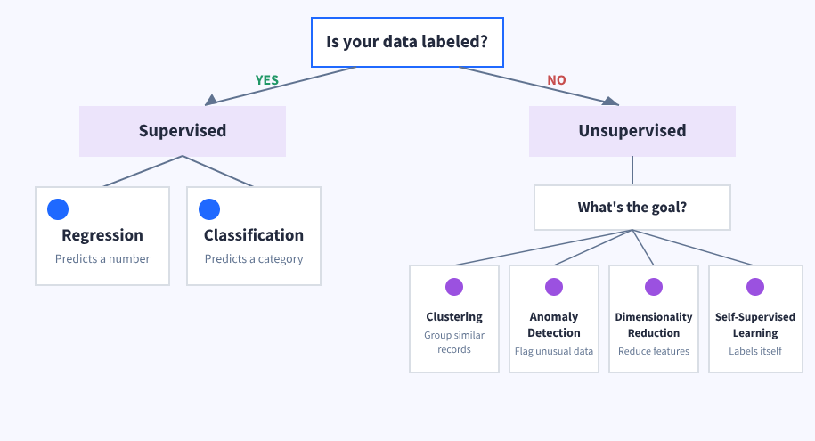
- Supervised learning trains an algorithm on labeled data, inputs paired with the correct answer, so the resulting model learns to map one to the other. Predicting house prices from square footage, or flagging spam emails, are both supervised problems because you have historical examples with known outcomes.
- Unsupervised learning trains an algorithm on unlabeled data. The resulting model finds structure on its own, grouping similar records together without being told what the groups should be. Customer segmentation is a common example.
- Semi-supervised learning trains an algorithm on a small set of labeled examples plus a much larger pool of unlabeled data, which is useful when labeling data is expensive or slow.
- Self-supervised learning generates its own labels from the structure of the data itself, often by hiding part of an input and training the model to predict it. It's the main pretraining approach behind most large language models, though later training stages often bring in other training methods.
- Reinforcement learning trains an algorithm through trial and error, rewarding actions that move toward a goal and penalizing ones that don't. It's how systems learn to play games or control robots.
Most of the models covered in this guide are trained using supervised or unsupervised learning, so that's where this guide focuses. Within supervised learning, models are typically built to solve one of two tasks: regression, which predicts a number, or classification, which predicts a category.
A note on the code in this guide: every snippet below is a minimal example. The supervised examples assume
X_train,X_test,y_train, andy_testalready exist and are reasonably clean, while the clustering example usesX. In a real project, you'd also handle missing data, encode categorical variables, and scale features where appropriate, especially for KNN, logistic regression, ridge, lasso, SVMs, and k-means, since tree-based models are generally much less sensitive to feature scale. Hyperparameters should be tuned using validation data or cross-validation rather than the training data alone.
Regression Models
Regression models predict a numeric quantity, often continuous, like a price, a temperature, or a duration. That's a different question from whether your target is stored as a number. Values like 0, 1, and 2 can still represent categories rather than quantities, so it's the meaning of the target that determines whether you're solving a regression or classification problem, not just its data type.
1. Linear Regression
Linear regression finds the straight line that best fits the relationship between an input variable and your target, or, once you add more inputs, a linear surface fit across all of them. If you're predicting a house's rental price from its size, bedroom count, and furnishing status, linear regression estimates how these factors combine to produce the final number.
The model finds this fit by minimizing the total squared distance between its predictions and the actual values in your training data, a method called least squares. The result is an interpretable model.
Its coefficients describe how the prediction changes with each feature, holding the other included features constant. How you read them, though, depends on how your features are scaled and how correlated they are with each other.
from sklearn.linear_model import LinearRegression

# X_train holds features like size, bedrooms, furnished (0/1)
# y_train holds the known rental prices
model = LinearRegression()
model.fit(X_train, y_train)

predictions = model.predict(X_test)
2. Ridge Regression
Plain linear regression has a weakness. When it's trained on data with many correlated features, its coefficients can become unstable and high-variance, which can sometimes hurt how well the model performs on new data. Ridge regression addresses this by adding a penalty that discourages large coefficients, generally shrinking them toward zero without forcing them all the way there.
from sklearn.linear_model import Ridge

ridge_model = Ridge(alpha=1.0)
ridge_model.fit(X_train, y_train)
ridge_predictions = ridge_model.predict(X_test)
3. Lasso Regression
Lasso regression addresses the same correlated-feature problem as ridge, but its penalty works differently as it increases. It can push a coefficient all the way to zero, effectively removing that feature from the model.
That makes lasso useful for feature selection, though when features are correlated, which ones get zeroed out can be somewhat unstable. Treat the result as a useful signal rather than a definitive list of what matters.
from sklearn.linear_model import Lasso

lasso_model = Lasso(alpha=1.0)
lasso_model.fit(X_train, y_train)
lasso_predictions = lasso_model.predict(X_test)
How Regression Models Are Evaluated
Standard classification accuracy doesn't apply to regression, since regression produces numeric predictions rather than discrete classes to get right or wrong. Instead, regression models are usually evaluated with error-based metrics that measure how far predictions land from the real values.
| Metric | What It Measures | Notes |
|---|---|---|
| MAE (Mean Absolute Error) | Average absolute distance between predicted and actual values | Penalizes errors linearly rather than squaring them |
| MSE (Mean Squared Error) | Average squared distance between predicted and actual values | Penalizes large errors more heavily |
| RMSE (Root Mean Squared Error) | Square root of MSE | Returned in the same unit as your target, so it's easier to interpret than MSE |
Classification Models
Classification models predict a category instead of a number. If your target has two possible outcomes, spam or not spam, approve or deny, that's binary classification. Three or more possible outcomes, like identifying which of several animal species is in a photo, makes it a multiclass problem.
4. Logistic Regression
Despite the name, logistic regression is a classification algorithm, not a regression one. In binary classification, it applies an S-shaped sigmoid function to estimate the probability of the positive class, mapping any input to a value between 0 and 1; for multiclass problems, common implementations instead use a softmax function to estimate a probability for each class.
For a spam filter, an email with several suspicious keywords might get a predicted probability of 0.92, which gets compared against a threshold, usually 0.5 by default, to produce a final classification of "spam." You can adjust that threshold depending on how costly false positives are for your use case.
from sklearn.linear_model import LogisticRegression

log_reg = LogisticRegression()
log_reg.fit(X_train, y_train)
predictions = log_reg.predict(X_test)
5. K-Nearest Neighbors (KNN)
KNN classifies a new data point by looking at the "k" closest points to it in the training data and assigning it to whichever class is most common among them. If k is 5 and four of the five nearest neighbors belong to Class A, the new point gets classified as Class A.
The choice of k matters. A small value makes the model sensitive to noise and outliers, while a large value can smooth over meaningful distinctions between classes. Most practitioners test several values of k and pick the one that performs best on validation data.
from sklearn.neighbors import KNeighborsClassifier

knn = KNeighborsClassifier(n_neighbors=5)
knn.fit(X_train, y_train)
predictions = knn.predict(X_test)
6. Naive Bayes
Naive Bayes applies probability theory under the simplifying assumption that features are independent given the class, an assumption that's rarely completely true, but the method still performs surprisingly well on tasks like text classification and spam filtering.
from sklearn.naive_bayes import GaussianNB

nb = GaussianNB()
nb.fit(X_train, y_train)
predictions = nb.predict(X_test)
7. Support Vector Machines (SVM)
Support vector machines (SVMs) seek a decision boundary with the widest possible margin between classes. Soft-margin SVMs allow some classification errors rather than requiring a perfect split, and kernel functions let the model draw nonlinear boundaries, which is part of why SVMs can perform well on high-dimensional feature representations, such as TF-IDF text vectors, especially on smaller datasets.
from sklearn.svm import SVC

svm = SVC(kernel='rbf', random_state=42)
svm.fit(X_train, y_train)
predictions = svm.predict(X_test)
How Classification Models Are Evaluated
Accuracy, the percentage of predictions the model got right, is the metric people reach for first, but it can be misleading. If a rare disease affects 5% of patients, a model that predicts "no disease" for everyone would score 95% accuracy while catching zero actual cases.
That's why classification models are also evaluated on precision (how many predicted positives were correct) and recall (how many actual positives the model caught). Which one you prioritize depends on your use case.
A fraud detector may prioritize recall when missing fraud is especially costly, while still monitoring precision since false alarms create real operational costs. A content moderation system reviewing borderline posts, on the other hand, might favor precision to avoid over-flagging.
Tree-Based and Ensemble Models
Tree-based models work by splitting data into branches based on feature values, continuing until they reach a decision. They handle both regression and classification problems and are some of the most widely used models in applied machine learning.
8. Decision Trees
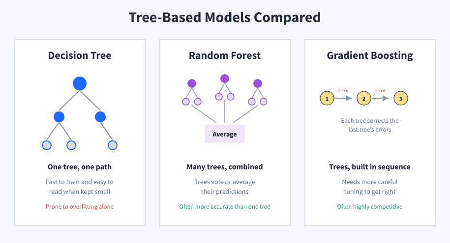
A decision tree repeatedly chooses a feature and threshold that most reduces impurity for a classification problem, or prediction error for a regression problem. It keeps splitting the data until it reaches terminal leaves that produce a final class, probability, or numeric prediction.
Small trees are relatively easy to inspect and explain, which is a real advantage when you need to justify a model's decision to a non-technical stakeholder, though that advantage fades as a tree grows large and hard to trace.
The tradeoff is that a decision tree left to grow without limits will often overfit, memorizing quirks of the training data instead of learning patterns that generalize.
from sklearn.tree import DecisionTreeClassifier, DecisionTreeRegressor

# Classification
clf = DecisionTreeClassifier(max_depth=5, random_state=42)
clf.fit(X_train, y_train)
clf_predictions = clf.predict(X_test)

# Regression
reg = DecisionTreeRegressor(max_depth=5, random_state=42)
reg.fit(X_train, y_train)
reg_predictions = reg.predict(X_test)
9. Random Forests
A random forest trains many decision trees. Each tree is fitted to a bootstrap sample of the training rows, and at each split, the tree considers only a random subset of features rather than all of them. For classification, the forest combines the trees' predicted class probabilities, or, in some implementations, their individual class predictions; for regression, it averages their numeric outputs.
This combination, often called an ensemble, is what tends to make random forests more reliable than a single decision tree. Because the trees are trained on different bootstrap samples and feature subsets, their prediction errors are partly decorrelated, and averaging them often reduces variance.
That makes the forest more stable and less sensitive to small changes in the training data than one tree on its own, though a random forest can still overfit or underperform on a dataset it isn't well suited to.
from sklearn.ensemble import RandomForestClassifier

rf_clf = RandomForestClassifier(n_estimators=200, max_depth=8, random_state=42)
rf_clf.fit(X_train, y_train)
predictions = rf_clf.predict(X_test)
10. Gradient Boosting
Where random forests build trees independently and average them, gradient boosting builds trees one at a time, with each new tree correcting the errors of the ones before it. This sequential approach is common in production systems and machine learning competitions because it tends to produce highly accurate models.
It often needs more careful tuning than a random forest, though modern, histogram-based implementations can still train quickly even on large datasets.
Popular gradient-boosting implementations include XGBoost, LightGBM, CatBoost, and scikit-learn's own GradientBoostingClassifier and faster HistGradientBoostingClassifier estimators. Gradient boosting is worth learning once you're comfortable with decision trees and random forests.
| Model | Speed | Interpretability | Common Tendency |
|---|---|---|---|
| Decision Tree | Fast to train | High when kept small | Simplest, but prone to overfitting alone |
| Random Forest | Moderate | Low to moderate; usually needs feature-importance or other post-hoc tools | Often more accurate than a single tree |
| Gradient Boosting | Varies; modern implementations can be fast | Lower | Often competitive with or ahead of random forests, depending on tuning and dataset |
The best choice among the three depends heavily on your dataset size, feature types, and how much time you have for tuning; it's worth testing more than one rather than assuming a fixed ranking.
Clustering Models
So far, every model covered has been supervised, trained on data with known answers. Clustering flips that: it groups similar data points together without being told what the groups should represent.
11. K-Means Clustering
K-means is one of the most widely used clustering algorithms, and it works in a repeating cycle. It initializes a set of starting centroids, commonly using a smarter method called k-means++ rather than pure random placement.
It then assigns every data point to its nearest centroid, recalculates each centroid based on the points assigned to it, and repeats until the centroids stop moving much or it hits a set number of iterations.
Common uses include customer segmentation, where a retailer groups shoppers by purchasing behavior without predefining what those groups look like, and exploratory grouping more broadly.
K-means can also support simple anomaly detection by flagging observations that fall unusually far from their nearest centroid, though that requires choosing a separate distance threshold; k-means itself doesn't produce an "anomaly" label, since it assigns every observation to some cluster.
from sklearn.cluster import KMeans

kmeans = KMeans(n_clusters=4, init='k-means++', random_state=42)
kmeans.fit(X)
predictions = kmeans.labels_  # cluster assignment for each row in X
Choosing the right value for "k" isn't automatic. You typically compare several values using a technique called the elbow method, which plots the within-cluster sum of squares (also called inertia) against different values of k and looks for the point where adding more clusters stops meaningfully improving the fit.
The elbow isn't always obvious, though, so it's common to pair it with silhouette analysis or domain knowledge about how many groups actually make sense for your use case.
It's also worth knowing where k-means struggles: it tends to work best when clusters are compact, roughly spherical, and similar in size, and it can produce unintuitive groupings when clusters are elongated or vary widely in spread.
12. Neural Networks
Every model covered so far belongs to what's often called "classical" machine learning. Neural networks are a different, more flexible model family, one that can be applied to structured tabular data as well as unstructured data like images, audio, and text, though their clearest advantage tends to show up on the unstructured side, where a model benefits from learning its own representations directly from raw input.
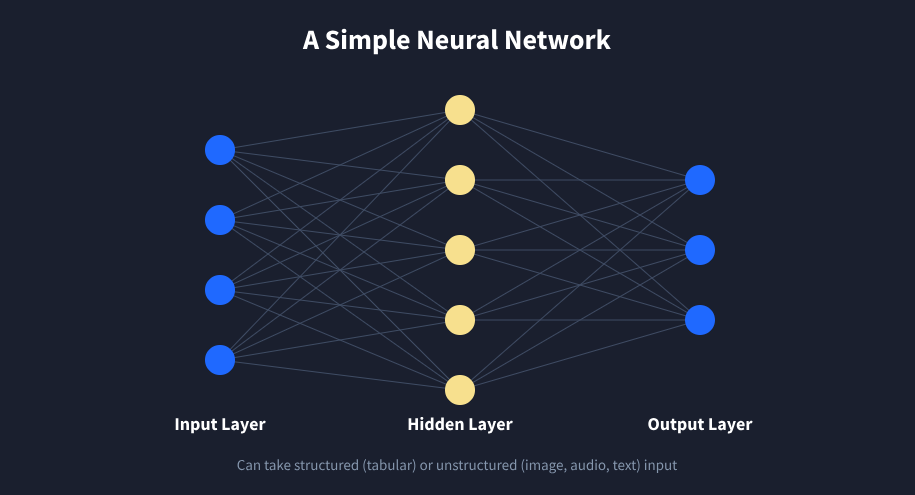
A neural network is built from layers of connected nodes, loosely modeled on how neurons pass signals. Each layer transforms its input and passes it forward.
With enough layers and data, the network can learn patterns that are hard to capture with a straight line or a set of tree splits, which is part of why neural networks power image recognition, speech-to-text, and the large language models behind tools like ChatGPT.
The tradeoff is cost. Neural networks generally need more data and computing power to train well, and they're harder to interpret than a decision tree or a linear regression model.
On many small-to-medium tabular datasets, tree-based ensembles like random forests and gradient boosting remain highly competitive and often train faster, so it's worth trying them first on structured business problems like churn prediction or pricing before reaching for a neural network.
That said, neural networks aren't limited to unstructured data. They're also used on tabular data, time series, and recommendation systems when the dataset and problem justify the added complexity.
Dataquest's Deep Learning in TensorFlow skill path and its Introduction to Deep Learning in PyTorch course pick up right where this guide leaves off, once you're ready to go deeper into this model family.
How to Choose the Right Machine Learning Model
With this many options, picking a starting point can feel harder than actually building the model. In practice, the decision usually comes down to four questions:
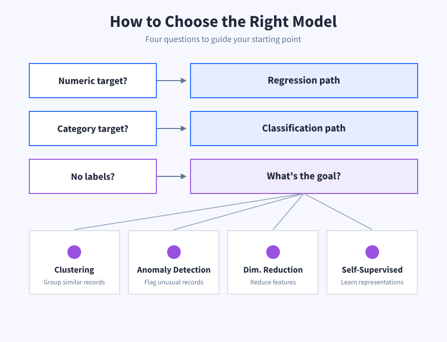
- Is your target a number or a category? Numbers point you toward regression models; categories point you toward classification models.
- Do you have labeled data? If not, you may need clustering, anomaly detection, dimensionality reduction, self-supervised learning, or another unlabeled-data approach, depending on what you want the model to accomplish.
- Does the model need to be explainable? A small decision tree or a linear or logistic model is generally easier to inspect and justify than a neural network, though explainability also depends on feature design, preprocessing, and how complex the final model ends up being.
- What kind of data are you working with? Structured tabular data often works well with linear or logistic models and tree-based ensembles. Raw images, audio, and text often benefit from neural networks, especially when the model needs to learn representations directly from the input, but classical models can still provide strong baselines, particularly for text represented with techniques like TF-IDF.
A reasonable default for most beginner and intermediate projects on tabular data is to start with a simple, interpretable model, linear or logistic regression, to establish a baseline, then move to a random forest or gradient boosting model if you need more accuracy.
Reach for a neural network once your data or problem genuinely calls for it, and compare it against a classical baseline rather than assuming it will win by default.
Machine Learning Models in the Real World
It's easier to see how these models fit together with a concrete scenario. A mid-sized e-commerce company wants to reduce customer churn, so a data analyst starts by pulling a year of purchase history, support tickets, and login activity into a single dataset.
The first model built is a logistic regression classifier, using "will this customer churn in the next 90 days" as the target. It may not turn out to be the most accurate option available, but it's fast to build.
Its coefficients give the team an early, conditional read on how factors like declining order frequency, a recent complaint, and a lapsed subscription are associated with churn, interpreted cautiously, since feature scale and correlation between predictors can distort how their raw size compares.
Once that baseline is in place, the team trains a random forest on the same data and finds it improves prediction accuracy by a meaningful margin, at the cost of losing some of that direct interpretability.
Alongside the churn model, the marketing team runs k-means clustering on customer purchase patterns to segment shoppers into groups for targeted campaigns, unrelated to the churn prediction itself but built from the same underlying data.
This kind of layered approach, a simple model for a baseline, a stronger model for production, and clustering for segmentation, shows up constantly in real data teams, and it's one reason why understanding several model types matters more than mastering just one.
Building a Career Around Machine Learning Models
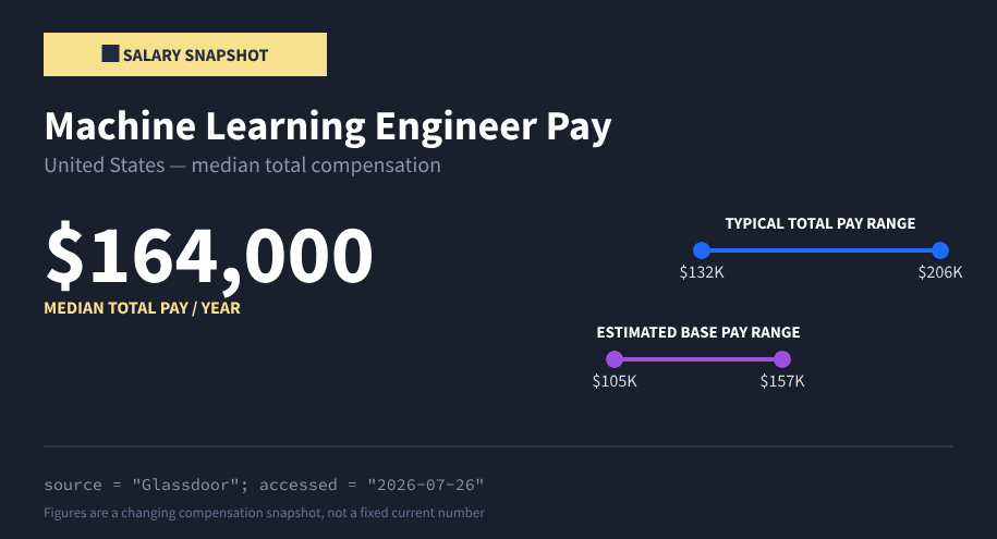
Understanding these models is also a practical career move. At the time of writing, Glassdoor's Machine Learning Engineer salary page lists median total pay for machine learning engineers in the United States at about $164,000 per year, with a typical total-pay range of roughly $131,000 to $206,000; estimated base pay is lower, at approximately $105,000 to $156,000. These figures were accessed on July 26, 2026.
Because Glassdoor's estimates change over time, treat them as a compensation snapshot rather than fixed current figures. Actual pay also varies by experience, location, employer, and specialization.
That said, getting there takes real, sustained practice, not a weekend of tutorials. Dataquest estimates its own Machine Learning Using Python skill path at roughly two months of study at five hours a week to build working knowledge of core models like the ones in this guide, though actual time varies a lot depending on your existing comfort with Python, statistics, and data analysis.
Getting to a job-ready level takes longer still, since machine learning roles also lean on skills like SQL, data cleaning, and increasingly, deployment and monitoring, not just model selection.
The good news is that you don't need to master every model type before you start being useful. For beginners, regression, classification, clustering, and tree-based models are practical starting points because they show up across many applied projects and establish concepts that transfer to more advanced methods.
Dataquest's Machine Learning Using Python path covers KNN, k-means, linear and logistic regression, decision trees, and random forests in sequence on real datasets, so the progression in this guide is one you can actually work through rather than just read about.
FAQ
What's the difference between a machine learning model and an algorithm?
An algorithm is the general procedure used to learn from data. A model is the specific result you get after that algorithm has been trained, the version that's ready to make predictions.
What's the difference between supervised and unsupervised learning?
Supervised learning trains a model on labeled data, inputs paired with the correct answer, so it learns to map one to the other, as in predicting house prices or flagging spam. Unsupervised learning trains on unlabeled data and finds structure on its own, as in grouping customers by purchasing behavior without predefined categories.
How many types of machine learning models are there?
There's no single official count, but machine learning models are usually grouped three ways: by how they learn, what they predict, and what family they belong to. Common learning settings include supervised, unsupervised, semi-supervised, self-supervised, and reinforcement learning.
Common tasks include regression, classification, clustering, anomaly detection, and dimensionality reduction. Model families include linear models, nearest-neighbor methods, tree-based ensembles, support vector machines, probabilistic models, and neural networks, and these families cut across tasks rather than lining up neatly with them.
Which machine learning model should I learn first?
Linear and logistic regression are common starting points, since they're simple to understand, quick to train, and directly connected to concepts like coefficients and probability that show up throughout machine learning.
Is random forest better than a decision tree?
Not automatically. A random forest usually generalizes better and is less sensitive to small changes in the training data than a single decision tree, but it's harder to interpret.
A well-tuned single tree can still be the right call when explainability matters more than squeezing out extra accuracy, and gradient boosting often edges out both on tabular data, though the best choice always depends on your dataset and how much tuning time you have.
Can the same algorithm be used for both classification and regression?
Yes. Decision trees, random forests, KNN, and neural networks can all be adapted to either type of problem, depending on whether the target variable is a category or a number.
Do I need to know advanced math to understand machine learning models?
Not to get started. You can build and use most of the models in this guide with a working understanding of the concepts and some comfort with Python, and pick up the underlying math as you go deeper into any specific model.
