Kaggle Competition: How I Ranked in the Top 15 with My First Attempt
Kaggle competitions are a fantastic way to learn data science and build your portfolio. I personally used Kaggle to learn many data science concepts. I started out with Kaggle a few months after learning basic Python programming, and later won several competitions. Doing well in a Kaggle competition requires more than just knowing all the latest machine learning algorithms―although that is helpful. Ultimately, it requires the right mindset, the willingness to learn, and a lot of data exploration. Many of these aspects aren't typically emphasized in tutorials on getting started with Kaggle, though. So in this post, I'll explain how I ranked in the top 15 of the Kaggle Expedia Hotel Recommendations competition by establishing the right mindset, setting up testing infrastructure, exploring the data, creating features, and making predictions. At the end, I'll show you how to generate a submission file using the techniques in the this post.
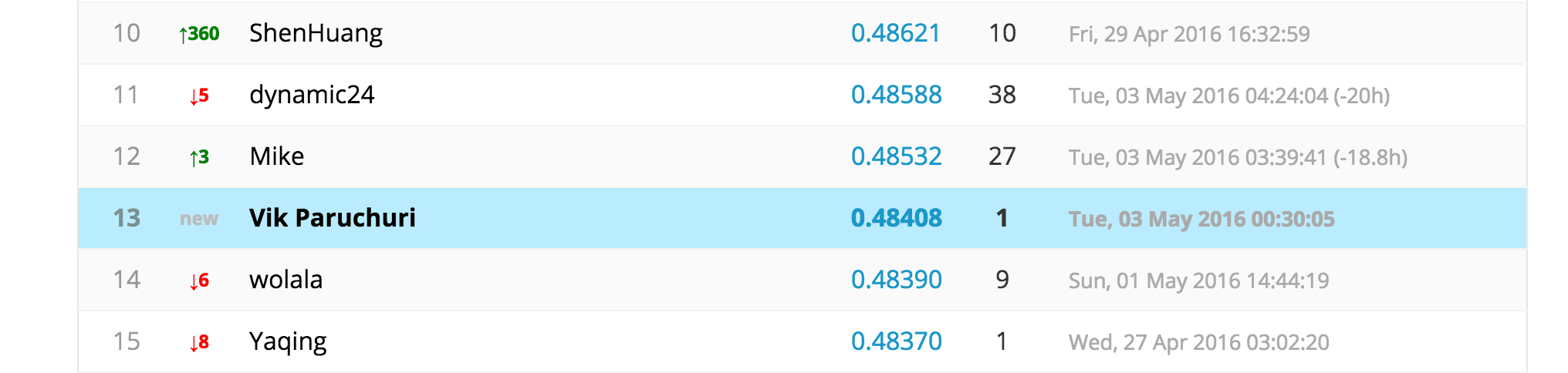
Where this submission ranked back in May of 2016.
The Expedia Hotel Recommendations Kaggle Competition
This Kaggle competition challenges you with predicting what hotel a user will book based on some attributes about the search the user is conducting on Expedia. Before we get into any of the coding, we'll need to put in some time to understand both the problem we're trying to solve and the data we'll use to do so.
A Quick Glance at the Columns
The first step is to look at the description of the columns of the dataset. You can find that here. Towards the bottom of the page, you'll see a description of each column in the data. Looking this over, it appears that we have quite a bit of data about the searches users are conducting on Expedia, along with data on what hotel cluster they eventually booked. This information is stored in the test.csv and train.csv files. The destinations.csv file contains information about the regions users searched for hotels. For now, we won't worry about what we're going to be predicting, and instead we'll focus on understanding the columns of the dataset first.
Expedia
Since the Kaggle competition consists of event data from users booking hotels on Expedia, we'll need to spend some time understanding the Expedia site. Understanding the booking flow will help us contextualize the fields in the dataset, and how they tie into using Expedia.

Above is how Expedia looked back in 2016 but the relationships described below still function similarly today.
Connection between the Site and the Kaggle Dataset
The textboxes in the screenshot above are connected to the Kaggle dataset in the following ways:
Going tomaps to thesrch_destination_type_id,hotel_continent,hotel_country, andhotel_marketfields in the dataset.Check-inmaps to thesrch_cifield in the datasetCheck-outmaps to thesrch_cofield in the dataset.Guestsmaps to thesrch_adults_cnt,srch_children_cnt, andsrch_rm_cntfields in the dataset.Add a flightmaps to theis_packagefield in the dataset.
The following attributes are determined by where the user is located, what device they're using, and details of their current Expedia session:
user_location_countryuser_location_regionuser_location_cityis_mobilechannelis_bookingcnt
Note: site_name is the name of the site you visited, whether it be the main Expedia.com site, or another one like Expedia.co.uk or Expedia.co.jp.
Just by looking at that one Expedia search screen, we can immediately contextualize a lot the important variables in the Kaggle dataset. Playing around with the Expedia search screen, filling in values, and going through the booking process can help further contextualize the variables.
The Kaggle Competition Dataset
Now that we have a handle on the data at a high level, we're ready to do some deeper exploration.
Downloading the Dataset
You can download the dataset for this Kaggle competition here. The datasets are fairly large, so you'll need a good chunk of disk space for them. You'll also need space to unzip the files to get the raw .csv version of the files instead of the compressed .csv.gz one.
Exploring the Dataset with Pandas
Given the amount of memory on your system, it may or may not be possible to read all the data in at once. If there isn't enough memory on your system, you should consider creating a machine on EC2 or DigitalOcean to process the data with.
Check out my tutorial on how to set up Docker for data science for help with this. Once we download the data, we can read it in using Pandas:
import pandas as pd

destinations = pd.read_csv("destinations.csv")
test = pd.read_csv("test.csv")
train = pd.read_csv("train.csv")
Let's first look at how much data there is:
train.shape(37670293, 24)test.shape(2528243, 22)We have almost 38 million rows of data in the training set, and about 2.5 million rows of data in the testing set. Working with all that data will make this problem a bit challenging! Let's explore the first few rows of the training data to see what we're dealing with:
train.head(5)| date_time | site_name | posa_continent | user_location_country | user_location_region | user_location_city | orig_destination_distance | user_id | is_mobile | is_package | ... | srch_children_cnt | srch_rm_cnt | srch_destination_id | srch_destination_type_id | is_booking | cnt | hotel_continent | hotel_country | hotel_market | hotel_cluster | |
|---|---|---|---|---|---|---|---|---|---|---|---|---|---|---|---|---|---|---|---|---|---|
| 0 | 2014-08-11 07:46:59 | 2 | 3 | 66 | 348 | 48862 | 2234.2641 | 12 | 0 | 1 | ... | 0 | 1 | 8250 | 1 | 0 | 3 | 2 | 50 | 628 | 1 |
| 1 | 2014-08-11 08:22:12 | 2 | 3 | 66 | 348 | 48862 | 2234.2641 | 12 | 0 | 1 | ... | 0 | 1 | 8250 | 1 | 1 | 1 | 2 | 50 | 628 | 1 |
| 2 | 2014-08-11 08:24:33 | 2 | 3 | 66 | 348 | 48862 | 2234.2641 | 12 | 0 | 0 | ... | 0 | 1 | 8250 | 1 | 0 | 1 | 2 | 50 | 628 | 1 |
| 3 | 2014-08-09 18:05:16 | 2 | 3 | 66 | 442 | 35390 | 913.1932 | 93 | 0 | 0 | ... | 0 | 1 | 14984 | 1 | 0 | 1 | 2 | 50 | 1457 | 80 |
| 4 | 2014-08-09 18:08:18 | 2 | 3 | 66 | 442 | 35390 | 913.6259 | 93 | 0 | 0 | ... | 0 | 1 | 14984 | 1 | 0 | 1 | 2 | 50 | 1457 | 21 |
There are a few things that immediately stick out for me in the training data:
- The
date_timecolumn could be useful in our predictions, so we'll need to ensure it's properly converted to the right data type before we can work with it. - Most of the other columns are integers or floats, so we can't do a lot of feature engineering. For example,
user_location_countryisn't the actual name of a country; it's an integer. This makes it harder to create new features, because we don't know exactly which country each value represents.
Now let's see what exploring the testing set can tell us about the data:
test.head(5)| id | date_time | site_name | posa_continent | user_location_country | user_location_region | user_location_city | orig_destination_distance | user_id | is_mobile | ... | srch_ci | srch_co | srch_adults_cnt | srch_children_cnt | srch_rm_cnt | srch_destination_id | srch_destination_type_id | hotel_continent | hotel_country | hotel_market | |
|---|---|---|---|---|---|---|---|---|---|---|---|---|---|---|---|---|---|---|---|---|---|
| 0 | 0 | 2015-09-03 17:09:54 | 2 | 3 | 66 | 174 | 37449 | 5539.0567 | 1 | 1 | ... | 2016-05-19 | 2016-05-23 | 2 | 0 | 1 | 12243 | 6 | 6 | 204 | 27 |
| 1 | 1 | 2015-09-24 17:38:35 | 2 | 3 | 66 | 174 | 37449 | 5873.2923 | 1 | 1 | ... | 2016-05-12 | 2016-05-15 | 2 | 0 | 1 | 14474 | 7 | 6 | 204 | 1540 |
| 2 | 2 | 2015-06-07 15:53:02 | 2 | 3 | 66 | 142 | 17440 | 3975.9776 | 20 | 0 | ... | 2015-07-26 | 2015-07-27 | 4 | 0 | 1 | 11353 | 1 | 2 | 50 | 699 |
| 3 | 3 | 2015-09-14 14:49:10 | 2 | 3 | 66 | 258 | 34156 | 1508.5975 | 28 | 0 | ... | 2015-09-14 | 2015-09-16 | 2 | 0 | 1 | 8250 | 1 | 2 | 50 | 628 |
| 4 | 4 | 2015-07-17 09:32:04 | 2 | 3 | 66 | 467 | 36345 | 66.7913 | 50 | 0 | ... | 2015-07-22 | 2015-07-23 | 2 | 0 | 1 | 11812 | 1 | 2 | 50 | 538 |
There are a few things we can take away from looking at the testing set:
- It looks like all the dates in
test.csvare later than the dates intrain.csv, and the data page confirms this―the testing set is from2015, and the training set is from2013and2014. - It looks like the user ids in
test.csvare a subset of the user ids intrain.csv, given the overlapping integer ranges. We can confirm this later on. - The
is_bookingcolumn always looks to be1intest.csv, and the data page confirms this.
Kaggle Competition Specifics
Before we go any further, we need to clearly define a couple of the key aspects of the competition.
What We're Predicting
We'll be predicting which hotel_cluster a user will book, given their search details. According to the description, there are 100 hotel clusters in total.
How Our Solution Is Scored
The evaluation page for this Kaggle competition says that we'll be scored using Mean Average Precision @ 5, which means that we'll need to make 5 cluster predictions for each row, and will be scored on whether or not the correct prediction appears in our list. If the correct prediction comes earlier in the list, we get more points. For example, if the "correct" cluster is 3, and we predict 4, 43, 60, 3, 20, our score will be lower than if we predict 3, 4, 43, 60, 20. This implies we should put predictions we're more certain about earlier in our list of predictions.
Exploring Hotel Clusters
Now that we know what we're predicting and how we'll be judged, it's time to dive in and really get to know our target column: hotel_cluster. We can use the value_counts method on a hotel_cluster Series object to do this:
train["hotel_cluster"].value_counts()
91    1043720
41     772743
48     754033
64     704734
65     670960
5      620194
       ...
53     134812
88     107784
27     105040
74      48355
The output above is truncated, but it shows that the number of hotels in each cluster is fairly evenly distributed. There doesn't appear to be any relationship between cluster number and the number of items.
Exploring Train and Test User IDs
Finally, let's confirm our hypothesis that all the test user ids are found in the train DataFrame. We can do this by finding the unique values for user_id in test, and seeing if they all exist in train. In the code below, we'll:
- Create a set of all the unique
testuser ids. - Create a set of all the unique
trainuser ids. - Figure out how many
testuser ids are in thetrainuser ids. - See if the count matches the total number of
testuser ids.
test_ids = set(test.user_id.unique())
train_ids = set(train.user_id.unique())
intersection_count = len(test_ids & train_ids)
intersection_count == len(test_ids)TrueLooks like our hypothesis is correct, which will make working with this data much easier!
Downsampling Our Kaggle Dataset
The entire train.csv dataset contains almost 38 million rows, which makes it hard to experiment with different techniques. Ideally, we want a small enough dataset that lets us quickly iterate through different approaches but is still representative of the whole training data. We can do this by first randomly sampling rows from our data, then selecting new training and testing datasets from train.csv. By selecting both sets from train.csv, we'll have the true hotel_cluster label for every row, and we'll be able to calculate our accuracy as we test techniques.
Extract Dates and Times
The first step is to add month and year fields to train. Because the train and test data is differentiated by date, we'll need to add date fields to allow us to segment our data into two sets the same way. If we add year and month fields, we can split our data into training and testing sets using them. The code below will:
- Convert the
date_timecolumn intrainfrom anobjectto adatetimevalue. This makes it easier to work with as a date. - Extract the
yearandmonthfrom thedate_timecolumn, and assign them to their own columns.
train["date_time"] = pd.to_datetime(train["date_time"])
train["year"] = train["date_time"].dt.year
train["month"] = train["date_time"].dt.month
Pick 10,000 Users
Because the user ids in test are a subset of the user ids in train, we'll need to do our random sampling in a way that preserves the full data of each user. We can accomplish this by selecting a certain number of users randomly, then only picking rows from train where user_id is in our random sample of user ids.
import random

unique_users = train.user_id.unique()

sel_user_id = random.sample(unique_user_id, 10000)
sel_train = train[train.user_id.isin(sel_user_ids)]
The above code creates a DataFrame called sel_train that only contains data from 10,000 users.
Create New, Smaller Training and Testing Sets
We'll now need to create new training and testing sets based on sel_train. We'll call these new datasets t1 and t2.
t1 = sel_train[((sel_train.year == 2013) | ((sel_train.year == 2014) & (sel_train.month < 8)))]
t2 = sel_train[((sel_train.year == 2014) & (sel_train.month >= 8))]
In the original train and test DataFrames, test contained data from 2015, and train contained data from 2013 and 2014. We split this data so that anything after July 2014 is in t2, and anything before is in t1. This gives us smaller training and testing sets with similar characteristics to the full train and test datasets.
Remove Click Events
If is_booking is 0, it represents a click, and a 1 represents a booking. test contains only booking events, so we'll need to sample t2 to only contain bookings as well.
t2 = t2[t2.is_booking == True]A Simple Algorithm
The most simple technique we could try on this data is to find the most common clusters across the data, then use them as predictions. We can again use the value_counts method to help us here:
most_common_clusters = list(train.hotel_cluster.value_counts().head().index)The above code will give us a list of the 5 most common clusters in train. This is because the head method returns the first 5 rows by default, and the index attribute will return the index of the DataFrame, which is the hotel cluster after running the value_counts method.
Generating Predictions
We can turn most_common_clusters into a list of predictions by making the same prediction for each row.
predictions = [most_common_clusters for i in range(t2.shape[0])]This will create a list with as many elements as there are rows in t2. Each element will be equal to most_common_clusters.
Evaluating Error
In order to evaluate error, we'll first need to figure out how to compute Mean Average Precision. Luckily, Ben Hamner has written an implementation that can be found here. It can be installed as part of the ml_metrics package, and you can find installation instructions for it here. We can compute our error metric with the mapk method found in same ml_metrics package:
import ml_metrics as metrics

target = [[l] for l in t2["hotel_cluster"]]
metrics.mapk(target, predictions, k=5)
0.058020770920711007Our target needs to be in list of lists format for the mapk function to work, so we convert the hotel_cluster column of t2 into a list of lists. Then, we call mapk by passing our target, our predictions, and the number of predictions we want to evaluate (5). Our result here isn't great, but we've just generated our first set of predictions, and evaluated our error! The framework we've built will allow us to quickly test out a variety of techniques and see how they score. We're well on our way to building a good-performing solution for the leaderboard.
Finding Correlations
Before we move on to creating a better algorithm, let's see if anything correlates well with hotel_cluster. This will tell us if we should dive more into any particular columns. We can find linear correlations in the training set using the corr method:
train.corr()["hotel_cluster"]
site_name                   -0.022408
posa_continent               0.014938
user_location_country       -0.010477
user_location_region         0.007453
user_location_city           0.000831
orig_destination_distance    0.007260
user_id                      0.001052
is_mobile                    0.008412
is_package                   0.038733
channel                      0.000707
This tells us that no columns correlate linearly with hotel_cluster. This makes sense, because there is no linear ordering to hotel_cluster. For example, having a higher cluster number isn't tied to having a higher srch_destination_id. Unfortunately, this means that techniques like linear regression and logistic regression won't work well on our data, because they rely on linear correlations between predictors and targets.
Creating Better Predictions for Our Kaggle Entry
This data for this competition is quite difficult to make predictions on using machine learning for a few reasons:
- There are millions of rows, which increases runtime and memory usage for algorithms.
- There are
100different clusters, and according to the competition admins, the boundaries are fairly fuzzy, so it will likely be hard to make predictions. As the number of clusters increases, classifiers generally decrease in accuracy. - Nothing is linearly correlated with the target (
hotel_clusters), meaning we can't use fast machine learning techniques like linear regression.
For these reasons, machine learning probably won't work well on our data, but we can try an algorithm and find out.
Generating Features
The first step in applying machine learning is to generate features. We can generate features using both what's available in the training data, and what's available in destinations. We haven't looked at destinations yet, so let's take a quick peek.
Generating Features from Destinations
Destinations contains an id that corresponds to srch_destination_id, along with 149 columns of latent information about that destination. Here's a sample:
| srch_destination_id | d1 | d2 | d3 | d4 | d5 | d6 | d7 | d8 | d9 | ... | d140 | d141 | d142 | d143 | d144 | d145 | d146 | d147 | d148 | d149 | |
|---|---|---|---|---|---|---|---|---|---|---|---|---|---|---|---|---|---|---|---|---|---|
| 0 | 0 | -2.198657 | -2.198657 | -2.198657 | -2.198657 | -2.198657 | -1.897627 | -2.198657 | -2.198657 | -1.897627 | ... | -2.198657 | -2.198657 | -2.198657 | -2.198657 | -2.198657 | -2.198657 | -2.198657 | -2.198657 | -2.198657 | -2.198657 |
| 1 | 1 | -2.181690 | -2.181690 | -2.181690 | -2.082564 | -2.181690 | -2.165028 | -2.181690 | -2.181690 | -2.031597 | ... | -2.165028 | -2.181690 | -2.165028 | -2.181690 | -2.181690 | -2.165028 | -2.181690 | -2.181690 | -2.181690 | -2.181690 |
| 2 | 2 | -2.183490 | -2.224164 | -2.224164 | -2.189562 | -2.105819 | -2.075407 | -2.224164 | -2.118483 | -2.140393 | ... | -2.224164 | -2.224164 | -2.196379 | -2.224164 | -2.192009 | -2.224164 | -2.224164 | -2.224164 | -2.224164 | -2.057548 |
| 3 | 3 | -2.177409 | -2.177409 | -2.177409 | -2.177409 | -2.177409 | -2.115485 | -2.177409 | -2.177409 | -2.177409 | ... | -2.161081 | -2.177409 | -2.177409 | -2.177409 | -2.177409 | -2.177409 | -2.177409 | -2.177409 | -2.177409 | -2.177409 |
| 4 | 4 | -2.189562 | -2.187783 | -2.194008 | -2.171153 | -2.152303 | -2.056618 | -2.194008 | -2.194008 | -2.145911 | ... | -2.187356 | -2.194008 | -2.191779 | -2.194008 | -2.194008 | -2.185161 | -2.194008 | -2.194008 | -2.194008 | -2.188037 |
The competition doesn't tell us exactly what each latent feature is, but it's safe to assume that it's some combination of destination characteristics, like name, description, and more. These latent features were converted to numbers, so they could be anonymized. We can use the destination information as features in a machine learning algorithm, but we'll need to compress the number of columns down first, to minimize runtime.
We can use PCA to do this. PCA will reduce the number of columns in a matrix while trying to preserve the same amount of variance per row. Ideally, PCA will compress all the information contained in all the columns into less, but in practice, some information is lost. In the code below, we:
- Initialize a PCA model using scikit-learn.
- Specify that we want to only have
3columns in our data. - Transform the columns
d1-d149into3columns.
from sklearn.decomposition import PCA

pca = PCA(n_components=3)
dest_small = pca.fit_transform(destinations[["d{0}".format(i + 1) for i in range(149)]])
dest_small = pd.DataFrame(dest_small)
dest_small["srch_destination_id"] = destinations["srch_destination_id"]
The above code compresses the 149 columns in destinations down to 3 columns, and creates a new DataFrame called dest_small. We preserve most of the variance in destinations while doing this, so we don't lose a lot of information, but save a lot of runtime for a machine learning algorithm.
Generating New Features
Now that the preliminaries are done with, we can generate our features. We'll do the following:
- Generate new date features based on
date_time,srch_ci, andsrch_co. - Remove non-numeric columns like
date_time. - Add in features from
dest_small. - Replace any missing values with
-1.
def calc_fast_features(df):
    df["date_time"] = pd.to_datetime(df["date_time"])
    df["srch_ci"] = pd.to_datetime(df["srch_ci"], format='
    df["srch_co"] = pd.to_datetime(df["srch_co"], format='

    props = {}
    for prop in ["month", "day", "hour", "minute", "dayofweek", "quarter"]:
        props[prop] = getattr(df["date_time"].dt, prop)

    carryover = [p for p in df.columns if p not in ["date_time", "srch_ci", "srch_co"]]
    for prop in carryover:
        props[prop] = df[prop]

    date_props = ["month", "day", "dayofweek", "quarter"]
    for prop in date_props:
        props["ci_{0}".format(prop)] = getattr(df["srch_ci"].dt, prop)
        props["co_{0}".format(prop)] = getattr(df["srch_co"].dt, prop)
    props["stay_span"] = (df["srch_co"] - df["srch_ci"]).astype('timedelta64[h]')

    ret = pd.DataFrame(props)

    ret = ret.join(dest_small, on="srch_destination_id", how='left', rsuffix="dest")
    ret = ret.drop("srch_destination_iddest", axis=1)
    return ret

df = calc_fast_features(t1)
df.fillna(-1, inplace=True)
The above will calculate features such as length of stay, check in day, and check out month. These features will help us train a machine learning algorithm later on. Replacing missing values with -1 isn't the best choice, but it will work fine for now, and we can always optimize the behavior later on.
Implementing a Machine Learning Algorithm
Now that we have features for our training data, we can try implementing some machine learning. We'll use 3-fold cross validation on the training set to generate a reliable error estimate. Cross validation splits the training set up into 3 parts, then predicts hotel_cluster for each part using the other parts to train with. We'll generate predictions using the Random Forest algorithm. Random forests build trees, which can fit to data with nonlinear tendencies. This will enable us to make predictions, even though none of our columns are linearly related. We'll first initialize the model and compute cross validation scores:
from sklearn import cross_validation
from sklearn.ensemble import RandomForestClassifier

predictors = [c for c in df.columns if c not in ["hotel_cluster"]]
clf = RandomForestClassifier(n_estimators=10, min_weight_fraction_leaf=0.1)
scores = cross_validation.cross_val_score(clf, df[predictors], df['hotel_cluster'], cv=3)
scores
array([ 0.06203556, 0.06233452, 0.06392277])The above code doesn't give us very good accuracy, and confirms our original suspicion that machine learning isn't a great approach to this problem. However, classifiers tend to have lower accuracy when there is a high cluster count. We can instead try training 100 binary classifiers. Each classifier will just determine if a row is in it's cluster, or not. This will entail training one classifier per label in hotel_cluster.
Binary Classifiers
We'll again train Random Forests, but each forest will predict only a single hotel cluster. We'll use 2 fold cross validation for speed, and only train 10 trees per label. In the code below, we:
- Loop across each unique
hotel_cluster.- Train a Random Forest classifier using 2-fold cross validation.
- Extract the probabilities from the classifier that the row is in the unique
hotel_cluster
- Combine all the probabilities.
- For each row, find the
5largest probabilities, and assign thosehotel_clustervalues as predictions. - Compute accuracy using
mapk.
from sklearn.ensemble import RandomForestClassifier
from sklearn.cross_validation import KFold
from itertools import chain

all_probs = []
unique_clusters = df["hotel_cluster"].unique()
for cluster in unique_clusters:
    df["target"] = 1
    df["target"][df["hotel_cluster"] != cluster] = 0
    predictors = [col for col in df if col not in ['hotel_cluster', "target"]]
    probs = []
    cv = KFold(len(df["target"]), n_folds=2)
    clf = RandomForestClassifier(n_estimators=10, min_weight_fraction_leaf=0.1)
    for i, (tr, te) in enumerate(cv):
        clf.fit(df[predictors].iloc[tr], df["target"].iloc[tr])
        preds = clf.predict_proba(df[predictors].iloc[te])
        probs.append([p[1] for p in preds])
    full_probs = chain.from_iterable(probs)
    all_probs.append(list(full_probs))

prediction_frame = pd.DataFrame(all_probs).T
prediction_frame.columns = unique_clusters
def find_top_5(row):
    return list(row.nlargest(5).index)

preds = []
for index, row in prediction_frame.iterrows():
    preds.append(find_top_5(row))

metrics.mapk([[l] for l in t2.iloc["hotel_cluster"]], preds, k=5)0.041083333333333326Our accuracy here is worse than before, and people on the leaderboard have much better accuracy scores. We'll need to abandon machine learning and move to the next technique in order to compete. Machine learning can be a powerful technique, but it isn't always the right approach to every problem.
Top Clusters Based on hotel_cluster
There are a few Kaggle Kernels for the competition that involve aggregating hotel_cluster based on orig_destination_distance, or srch_destination_id. Aggregating on orig_destination_distance will exploit a data leak in the competition, and attempt to match the same user together. Aggregating on srch_destination_id will find the most popular hotel clusters for each destination. We'll then be able to predict that a user who searches for a destination is going to one of the most popular hotel clusters for that destination. Think of this as a more granular version of the most common clusters technique we used earlier. We can first generate scores for each hotel_cluster in each srch_destination_id. We'll weight bookings higher than clicks. This is because the test data is all booking data, and this is what we want to predict. We want to include click information, but downweight it to reflect this. Step by step, we'll:
- Group
t1bysrch_destination_id, andhotel_cluster. - Iterate through each group, and:
- Assign 1 point to each hotel cluster where
is_bookingis True. - Assign
.15points to each hotel cluster whereis_bookingis False. - Assign the score to the
srch_destination_id/hotel_clustercombination in a dictionary.
- Assign 1 point to each hotel cluster where
Here's the code to accomplish the above steps:
def make_key(items):
    return "_".join([str(i) for i in items])

match_cols = ["srch_destination_id"]
cluster_cols = match_cols + ['hotel_cluster']
groups = t1.groupby(cluster_cols)
top_clusters = {}
for name, group in groups:
    clicks = len(group.is_booking[group.is_booking == False])
    bookings = len(group.is_booking[group.is_booking == True])

    score = bookings + .15 * clicks

    clus_name = make_key(name[:len(match_cols)])
    if clus_name not in top_clusters:
        top_clusters[clus_name] = {}
    top_clusters[clus_name][name[-1]] = score
At the end, we'll have a dictionary where each key is an srch_destination_id. Each value in the dictionary will be another dictionary, containing hotel clusters as keys with scores as values. Here's how it looks:
{'39331': {20: 1.15, 30: 0.15, 81: 0.3},
'511': {17: 0.15, 34: 0.15, 55: 0.15, 70: 0.15}}
We'll next want to transform this dictionary to find the top 5 hotel clusters for each srch_destination_id. In order to do this, we'll:
- Loop through each key in
top_clusters. - Find the top
5clusters for that key. - Assign the top
5clusters to a new dictionary,cluster_dict.
Here's the code:
import operator

cluster_dict = {}
for n in top_clusters:
    tc = top_clusters[n]
    top = [l[0] for l in sorted(tc.items(), key=operator.itemgetter(1), reverse=True)[:5]]
    cluster_dict[n] = top
Making Predictions Based on Destination
Once we know the top clusters for each srch_destination_id, we can quickly make predictions. To make predictions, all we have to do is:
- Iterate through each row in
t2.- Extract the
srch_destination_idfor the row. - Find the top clusters for that destination id.
- Append the top clusters to
preds.
- Extract the
Here's the code:
preds = []
for index, row in t2.iterrows():
    key = make_key([row[m] for m in match_cols])
    if key in cluster_dict:
        preds.append(cluster_dict[key])
    else:
        preds.append([])
At the end of the loop, preds will be a list of lists containing our predictions. It will look like this:
[
   [2, 25, 28, 10, 64],
   [25, 78, 64, 90, 60],
   ...
]
Calculating Error
Once we have our predictions, we can compute our accuracy using the mapk function from earlier:
metrics.mapk([[l] for l in t2["hotel_cluster"]], preds, k=5)0.22388136288998359We're doing pretty well! We boosted our accuracy 4x over the best machine learning approach, and we did it with a far faster and simpler approach. You may have noticed that this value is quite a bit lower than accuracies on the leaderboard. Local testing results in a lower accuracy value than submitting, so this approach will actually do fairly well on the leaderboard. Differences in leaderboard score and local score can come down to a few factors:
- Different data locally and in the hidden set that leaderboard scores are computed on. For example, we're computing error in a sample of the training set, and the leaderboard score is computed on the testing set.
- Techniques that result in higher accuracy with more training data. We're only using a small subset of data for training, and it may be more accurate when we use the full training set.
- Different randomization. With certain algorithms, random numbers are involved, but we're not using any of these.
Generating Better Predictions for your Kaggle Submission
The forums are very important in Kaggle, and can often help you find nuggets of information that will let you boost your score. The Expedia competition is no exception.
This post details a data leak that allows you to match users in the training set from the testing set using a set of columns including user_location_country, and user_location_region. We'll use the information from the post to match users from the testing set back to the training set, which will boost our score. Based on the forum thread, its okay to do this, and the competition won't be updated as a result of the leak.
Finding Matching Users
The first step is to find users in the training set that match users in the testing set. In order to do this, we need to:
- Split the training data into groups based on the match columns.
- Loop through the testing data.
- Create an index based on the match columns.
- Get any matches between the testing data and the training data using the groups.
Here's the code to accomplish this:
match_cols = ['user_location_country', 'user_location_region', 'user_location_city', 'hotel_market', 'orig_destination_distance']

groups = t1.groupby(match_cols)

def generate_exact_matches(row, match_cols):
    index = tuple([row[t] for t in match_cols])
    try:
        group = groups.get_group(index)
    except Exception:
        return []
    clus = list(set(group.hotel_cluster))
    return clus

exact_matches = []
for i in range(t2.shape[0]):
    exact_matches.append(generate_exact_matches(t2.iloc[i], match_cols))
At the end of this loop, we'll have a list of lists that contain any exact matches between the training and the testing sets. However, there aren't that many matches. To accurately evaluate error, we'll have to combine these predictions with our earlier predictions. Otherwise, we'll get a very low accuracy value, because most rows have empty lists for predictions.
Combining Predictions
We can combine different lists of predictions to boost accuracy. Doing so will also help us see how good our exact match strategy is. To do this, we'll have to:
- Combine
exact_matches,preds, andmost_common_clusters. - Only take the unique predictions, in sequential order, using the
f5function from here. - Ensure we have a maximum of
5predictions for each row in the testing set.
Here's how we can do it:
def f5(seq, idfun=None):
    if idfun is None:
        def idfun(x): return x
    seen = {}
    result = []
    for item in seq:
        marker = idfun(item)
        if marker in seen: continue
        seen[marker] = 1
        result.append(item)
    return result

full_preds = [f5(exact_matches[p] + preds[p] + most_common_clusters)[:5] for p in range(len(preds))]
mapk([[l] for l in t2["hotel_cluster"]], full_preds, k=5)
0.28400041050903119This is looking quite good in terms of error -- we improved dramatically from earlier! We could keep going and making more small improvements, but we're probably ready to submit now.
Making a Kaggle Submission file
Luckily, because of the way we wrote the code, all we have to do to submit our solution is assign train to the variable t1, and test to the variable t2. Then, we just have to re-run the code to make predictions. Re-running the code over the train and test sets should take less than an hour. Once we have predictions, we just have to write them to a file:
write_p = [" ".join([str(l) for l in p]) for p in full_preds]
write_frame = ["{0},{1}".format(t2["id"][i], write_p[i]) for i in range(len(full_preds))]
write_frame = ["id,hotel_clusters"] + write_frame
with open("predictions.csv", "w+") as f:
    f.write("\n".join(write_frame))
We'll then have a submission file in the right format to submit. Back when this post was first written in 2016, this particular submission would have placed you in the top 15.
Summary
We came a long way in this post! We went from just looking at the data all the way to creating a submission file that would have placed us on the leaderboard for this Kaggle competition. Along the way, some of the key steps we took were:
- Exploring the data and understanding the problem.
- Setting up a way to iterate quickly through different techniques.
- Creating a way to figure out accuracy locally.
- Reading the forums, scripts, and the descriptions of the contest very closely to better understand the structure of the data.
- Trying a variety of techniques and not being afraid to not use machine learning.
These steps will serve you well in any Kaggle competition.
Next Steps
In order to iterate quickly and explore techniques, speed is key. This is difficult with this competition, but there are a few strategies to try:
- Sampling down the data even more.
- Parallelizing operations across multiple cores.
- Using Spark or other tools where tasks can be run on parallel workers.
- Exploring various ways to write code and benchmarking to find the most efficient approach.
- Avoiding iterating over the full training and testing sets, and instead using groups.
Writing fast, efficient code is a huge advantage in this competition. Once you have a stable foundation on which to run your code, there are a few avenues to explore in terms of techniques to boost accuracy:
- Finding similarity between users, then adjusting hotel cluster scores based on similarity.
- Using similarity between destinations to group multiple destinations together.
- Applying machine learning within subsets of the data.
- Combining different prediction strategies in a less naive way.
- Exploring the link between hotel clusters and regions more.
I hope you have fun with this competition! If you want to learn more, check out our online data science courses to learn about data manipulation, statistics, machine learning, AI chatbots, deep learning, and more.
Looking for more about Kaggle? Check out these posts: