Kaggle Fundamentals: The Titanic Competition
Kaggle is a site where people create algorithms and compete against machine learning practitioners around the world. Your algorithm wins the competition if it's the most accurate on a particular data set. Kaggle is a fun way to practice your machine learning skills.
In this tutorial we'll learn learn how to:
- Approach a Kaggle competition
- Explore the competition data and learn about the competition topic
- Prepare data for machine learning
- Train a model
- Measure the accuracy of your model
- Prepare and make your first Kaggle submission
This tutorial presumes you have an understanding of Python and the pandas library. If you need to learn about these, we recommend our pandas tutorial blog post.
The Titanic competition
Kaggle has created a number of competitions designed for beginners. The most popular of these competitions, and the one we'll be looking at, is about predicting which passengers survived the sinking of the Titanic.
In this Titanic ML competition, we have data about passengers onboard the Titanic, and we'll see if we can use that information to predict whether those people survived or not. Before we start looking at this specific competition, let's take a moment to understand how Kaggle competitions work.
Each Kaggle competition has two key data files that you will work with - a training set and a testing set.
The training set contains data we can use to train our model. It has a number of feature columns which contain various descriptive data, as well as a column of the target values we are trying to predict: in this case, Survival.
The testing set contains all of the same feature columns, but is missing the target value column. Additionally, the testing set usually has fewer observations (rows) than the training set.

This is useful because we want as much data as we can to train our model on. Once we have trained our model on the training set, we will use that model to make predictions on the data from the testing set, and submit those predictions to Kaggle.
In this competition, the two files are named test.csv and train.csv. We'll start by using pandas.read_csv() to read both files and then inspect their size.
import pandas as pd

test = pd.read_csv("test.csv")
train = pd.read_csv("train.csv")
print("Dimensions of train: {}".format(train.shape))
print("Dimensions of test: {}".format(test.shape))
Dimensions of train: (891, 12)
Dimensions of test: (418, 11)
Exploring the data
The files we just opened are available on the data page for the Titanic competition on Kaggle. That page also has a data dictionary, which explains the various columns that make up the data set. Below are the descriptions contained in that data dictionary:
PassengerID— A column added by Kaggle to identify each row and make submissions easierSurvived— Whether the passenger survived or not and the value we are predicting (0=No, 1=Yes)Pclass— The class of the ticket the passenger purchased (1=1st, 2=2nd, 3=3rd)Sex— The passenger's sexAge— The passenger's age in yearsSibSp— The number of siblings or spouses the passenger had aboard the TitanicParch— The number of parents or children the passenger had aboard the TitanicTicket— The passenger's ticket numberFare— The fare the passenger paidCabin— The passenger's cabin numberEmbarked— The port where the passenger embarked (C=Cherbourg, Q=Queenstown, S=Southampton)
The data page on Kaggle has some additional notes about some of the columns. It's always worth exploring this in detail to get a full understanding of the data.
Let's take a look at the first few rows of the train dataframe.
train.head()The type of machine learning we will be doing is called classification, because when we make predictions we are classifying each passenger as 'survived' or not. More specifically, we are performing binary classification, which means that there are only two different states we are classifying.
In any machine learning exercise, thinking about the topic you are predicting is very important. We call this step acquiring domain knowledge, and it's one of the most important determinants for success in machine learning.
In this case, understanding the Titanic disaster and specifically what variables might affect the outcome of survival is important. Anyone who has watched the movie Titanic would remember that women and children were given preference to lifeboats (as they were in real life). You would also remember the vast class disparity of the passengers.
This indicates that Age, Sex, and PClass may be good predictors of survival. We'll start by exploring Sex and Pclass by visualizing the data.
Because the Survived column contains 0 if the passenger did not survive and 1 if they did, we can segment our data by sex and calculate the mean of this column. We can use DataFrame.pivot_table() to easily do this:
import matplotlib.pyplot as plt
%matplotlib inline

sex_pivot = train.pivot_table(index="Sex",values="Survived")
sex_pivot.plot.bar()
plt.show()
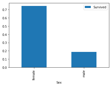
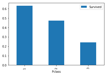
We can immediately see that females survived in much higher proportions than males did. Let's do the same with the Pclass column.
class_pivot = train.pivot_table(index="Pclass",values="Survived")
class_pivot.plot.bar()
plt.show()
Exploring and converting the age column
The Sex and PClass columns are what we call categorical features. That means that the values represented a few separate options (for instance, whether the passenger was male or female).
Let's take a look at the Age column using Series.describe().
train["Age"].describe()count 714.000000
mean 29.699118
std 14.526497
min 0.420000
25% 20.125000
50% 28.000000
75% 38.000000
max 80.000000
Name: Age, dtype: float64The Age column contains numbers ranging from 0.42 to 80.0 (If you look at Kaggle's data page, it informs us that Age is fractional if the passenger is less than one). The other thing to note here is that there are 714 values in this column, fewer than the 814 rows we discovered that the train data set had earlier which indicates we have some missing values.
All of this means that the Age column needs to be treated slightly differently, as this is a continuous numerical column. One way to look at distribution of values in a continuous numerical set is to use histograms. We can create two histograms to compare visually the those that survived vs those who died across different age ranges:
survived = train[train["Survived"] == 1]
died = train[train["Survived"] == 0]
survived["Age"].plot.hist(alpha=0.5,color='red',bins=50)
died["Age"].plot.hist(alpha=0.5,color='blue',bins=50)
plt.legend(['Survived','Died'])
plt.show()
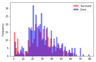
The relationship here is not simple, but we can see that in some age ranges more passengers survived - where the red bars are higher than the blue bars.
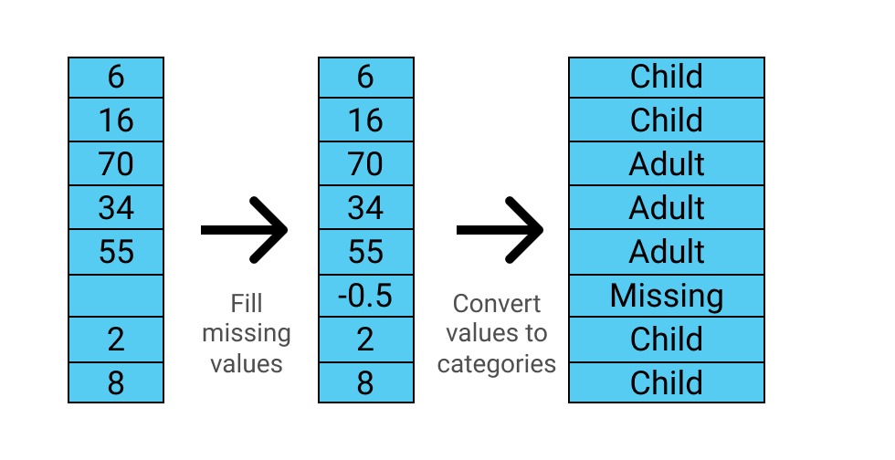
In order for this to be useful to our machine learning model, we can separate this continuous feature into a categorical feature by dividing it into ranges. We can use the pandas.cut() function to help us out.
The pandas.cut() function has two required parameters - the column we wish to cut, and a list of numbers which define the boundaries of our cuts. We are also going to use the optional parameter labels, which takes a list of labels for the resultant bins. This will make it easier for us to understand our results.
Before we modify this column, we have to be aware of two things. Firstly, any change we make to the train data, we also need to make to the test data, otherwise we will be unable to use our model to make predictions for our submissions. Secondly, we need to remember to handle the missing values we observed above.
We'll create a function that:
- Uses the
pandas.fillna()method to fill all of the missing values with-0.5 - Cuts the
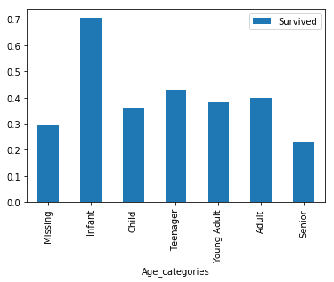
Agecolumn into six segments:Missing, from-1to0Infant, from0to5Child, from5to12Teenager, from12to18Young Adult, from18to35Adult, from35to60Senior, from60to100
We'll then use that function on both the train and test dataframes.
The diagram below shows how the function converts the data:
Note that the cut_points list has one more element than the label_names list, since it needs to define the upper boundary for the last segment.
def process_age(df,cut_points,label_names):
    df["Age"] = df["Age"].fillna(-0.5)
    df["Age_categories"] = pd.cut(df["Age"],cut_points,labels=label_names)
    return df

cut_points = [-1,0,5,12,18,35,60,100]
label_names = ["Missing","Infant","Child","Teenager","Young Adult","Adult","Senior"]
train = process_age(train,cut_points,label_names)
test = process_age(test,cut_points,label_names)

pivot = train.pivot_table(index="Age_categories",values='Survived')
pivot.plot.bar()
plt.show()
Preparing our data for machine learning
So far we have identified three columns that may be useful for predicting survival:
SexPclassAge, or more specifically our newly createdAge_categories
Before we build our model, we need to prepare these columns for machine learning. Most machine learning algorithms can't understand text labels, so we have to convert our values into numbers.
Additionally, we need to be careful that we don't imply any numeric relationship where there isn't one. The data dictionary tells us that the values in the Pclass columnare 1, 2, and 3. We can confirm this with pandas:
train["Pclass"].value_counts()3 491
1 216
2 184
Name: Pclass, dtype: int64
While the class of each passenger certainly has some sort of ordered relationship, the relationship between each class is not the same as the relationship between the numbers 1, 2, and 3. For instance, class 2 isn't "worth" double what class 1 is, and class 3 isn't "worth" triple what class 1 is.
In order to remove this relationship, we can create dummy columns for each unique value in Pclass:

Rather than doing this manually, we can use the pandas.get_dummies() function which will generate columns shown in the diagram above.
We'll create a function to create the dummy columns for the Pclass column and add it back to the original dataframe. We'll then apply that function on the train and test dataframes for each of the Pclass, Sex, and Age_categories columns.
def create_dummies(df,column_name):
    dummies = pd.get_dummies(df[column_name],prefix=column_name)
    df = pd.concat([df,dummies],axis=1)
    return df

for column in ["Pclass","Sex","Age_categories"]:
    train = create_dummies(train,column)
    test = create_dummies(test,column)
Creating our first machine learning model
Now that our data has been prepared, we are ready to train our first model. The first model we will use is called Logistic Regression, which is often the first model you will train when performing classification.
We will be using the scikit-learn library as it has many tools that make performing machine learning easier. The scikit-learn workflow consists of four main steps:
- Instantiate (or create) the specific machine learning model you want to use
- Fit the model to the training data
- Use the model to make predictions
- Evaluate the accuracy of the predictions
Each model in scikit-learn is implemented as a separate class and the first step is to identify the class we want to create an instance of. In our case, we want to use the LogisticRegression class.
We'll start by looking at the first two steps. First, we need to import the class:
from sklearn.linear_model import LogisticRegressionNext, we create a LogisticRegression object:
lr = LogisticRegression()Lastly, we use the LogisticRegression.fit() method to train our model. The .fit() method accepts two arguments: X and y. X must be a two dimensional array (like a dataframe) of the features that we wish to train our model on, and y must be a one-dimensional array (like a series) of our target, or the column we wish to predict.
columns = ['Pclass_2', 'Pclass_3', 'Sex_male']
lr.fit(train[columns], train['Survived'])
The code above fits (or trains) our LogisticRegression model using three columns: Pclass_2, Pclass_3, and Sex_male.
Let's train our model using all of the columns we created with our create_dummies() function.
from sklearn.linear_model import LogisticRegression

columns = ['Pclass_1', 'Pclass_2', 'Pclass_3', 'Sex_female', 'Sex_male',
       'Age_categories_Missing','Age_categories_Infant',
       'Age_categories_Child', 'Age_categories_Teenager',
       'Age_categories_Young Adult', 'Age_categories_Adult',
      'Age_categories_Senior']

lr = LogisticRegression()
lr.fit(train[columns], train["Survived"])
LogisticRegression(C=1.0, class_weight=None, dual=False, fit_intercept=True,
          intercept_scaling=1, max_iter=100, multi_class='ovr', n_jobs=1,
          penalty='l2', random_state=None, solver='liblinear', tol=0.0001,
          verbose=0, warm_start=False)
Splitting our training data
Congratulations, you've trained your first machine learning model! Our next step is to find out how accurate our model is, and to do that, we'll have to make some predictions.
If you recall from earlier, we do have a test dataframe that we could use to make predictions. We could make predictions on that data set, but because it doesn't have the Survived column we would have to submit it to Kaggle to find out our accuracy. This would quickly become a pain if we had to submit to find out the accuracy every time we optimized our model.
We could also fit and predict on our train dataframe, however if we do this there is a high likelihood that our model will overfit, which means it will perform well because we're testing on the same data we've trained on, but then perform much worse on new, unseen data.
Instead we can split our train dataframe into two:
- One part to train our model on (often 80% of the observations)
- One part to make predictions with and test our model (often 20% of the observations)
The convention in machine learning is to call these two parts train and test. This can become confusing, since we already have our test dataframe that we will eventually use to make predictions to submit to Kaggle. To avoid confusion, from here on, we're going to call this Kaggle 'test' data holdout data, which is the technical name given to this type of data used for final predictions.
The scikit-learn library has a handy model_selection.train_test_split() function that we can use to split our data. train_test_split() accepts two parameters, X and y, which contain all the data we want to train and test on, and returns four objects: train_X, train_y, test_X, test_y:

You'll notice that we use some extra parameters: test_size, which lets us control what proportions our data are split into, and random_state. The train_test_split() function randomizes observations before dividing them, and setting a random seed means that our results will be reproducible, so you can follow along and get the same result as we did.
holdout = test # from now on we will refer to this
               # dataframe as the holdout data

from sklearn.model_selection import train_test_split

all_X = train[columns]
all_y = train['Survived']

train_X, test_X, train_y, test_y = train_test_split(
    all_X, all_y, test_size=0.20,random_state=0)
Making predictions and measuring their accuracy
Now that we have our data split into train and test sets, we can fit our model again on our training set, and then use that model to make predictions on our test set.
Once we have fit our model, we can use the LogisticRegression.predict() method to make predictions.
The predict() method takes a single parameter X, a two dimensional array of features for the observations we wish to predict. X must have the exact same features as the array we used to fit our model. The method returns single dimensional array of predictions.
lr = LogisticRegression()
lr.fit(train_X, train_y)
predictions = lr.predict(test_X)
There are a number of ways to measure the accuracy of machine learning models, but when competing in Kaggle competitions you want to make sure you use the same method that Kaggle uses to calculate accuracy for that specific competition.
In this case, the evaluation section for the Titanic competition on Kaggle tells us that our score calculated as "the percentage of passengers correctly predicted". This is by far the most common form of accuracy for binary classification.
As an example, imagine we were predicting a small data set of five observations.
| Our model's prediction | The actual value | Correct |
|---|---|---|
| 0 | 0 | Yes |
| 1 | 0 | No |
| 0 | 1 | No |
| 1 | 1 | Yes |
| 1 | 1 | Yes |
In this case, our model correctly predicted three out of five values, so the accuracy based on this prediction set would be 60%.
Again, scikit-learn has a handy function we can use to calculate accuracy: metrics.accuracy_score(). The function accepts two parameters, y_true and y_pred, which are the actual values and our predicted values respectively, and returns our accuracy score.
from sklearn.metrics import accuracy_score

accuracy = accuracy_score(test_y, predictions)
Let's put all of these steps together, and get our first accuracy score.
from sklearn.metrics import accuracy_score

lr = LogisticRegression()
lr.fit(train_X, train_y)
predictions = lr.predict(test_X)
accuracy = accuracy_score(test_y, predictions)
print(accuracy)
0.810055865922Using cross validation for more accurate error measurement
Our model has an accuracy score of 81.0% when tested against our 20% test set. Given that this data set is quite small, there is a good chance that our model is overfitting, and will not perform as well on totally unseen data.
To give us a better understanding of the real performance of our model, we can use a technique called cross validation to train and test our model on different splits of our data, and then average the accuracy scores.

The most common form of cross validation, and the one we will be using, is called k-fold cross validation. 'Fold' refers to each different iteration that we train our model on, and 'k' just refers to the number of folds. In the diagram above, we have illustrated k-fold validation where k is 5.
We will use scikit-learn's model_selection.cross_val_score() function to automate the process. The basic syntax for cross_val_score() is:
cross_val_score(estimator, X, y, cv=None)estimatoris a scikit-learn estimator object, like theLogisticRegression()objects we have been creating.Xis all features from our data set.yis the target variables.cvspecifies the number of folds.
The function returns a numpy ndarray of the accuracy scores of each fold. It's worth noting, the cross_val_score() function can use a variety of cross validation techniques and scoring types, but it defaults to k-fold validation and accuracy scores for our input types.
We'll use model_selection.cross_val_score() to perform cross-validation on our data, before calculating the mean of the scores produced:
from sklearn.model_selection import cross_val_score

lr = LogisticRegression()
scores = cross_val_score(lr, all_X, all_y, cv=10)
scores.sort()
accuracy = scores.mean()

print(scores)
print(accuracy)
[ 0.76404494  0.76404494  0.7752809   0.78651685  0.8         0.80681818  0.80898876  0.81111111  0.83146067  0.87640449]
0.802467086596
Making predictions on unseen data
From the results of our k-fold validation, you can see that the accuracy number varies with each fold - ranging between 76.4% and 87.6%. This demonstrates why ccross-validationis important.
As it happens, our average accuracy score was 80.2%, which is not far from the 81.0% we got from our simple train/test split; however , this will not always be the case, and you should always use cross-validation to make sure the error metrics you are getting from your model are accurate.
We are now ready to use the model we have built to train our final model and then make predictions on our unseen holdout data, or what Kaggle calls the 'test' data set.
lr = LogisticRegression()
lr.fit(all_X,all_y)
holdout_predictions = lr.predict(holdout[columns])
Creating a submission file
The last thing we need to do is create a submission file. Each Kaggle competition can have slightly different requirements for the submission file. Here's what is specified on the Titanic competition evaluation page:
You should submit a csv file with exactly 418 entries plus a header row. Your submission will show an error if you have extra columns (beyond PassengerId and Survived) or rows.
The file should have exactly 2 columns:
- PassengerId (sorted in any order)
- Survived (contains your binary predictions: 1 for survived, 0 for deceased)
The table below shows this in a slightly easier to understand format, so we can visualize what we are aiming for.
| PassengerId | Survived |
|---|---|
| 892 | 0 |
| 893 | 1 |
| 894 | 0 |
We will need to create a new dataframe that contains the holdout_predictions we created in the previous screen and the PassengerId column from the holdout dataframe. We don't need to worry about matching the data up, as both of these remain in their original order.
To do this, we can pass a dictionary to the pandas.DataFrame() function:
holdout_ids = holdout["PassengerId"]
submission_df = {"PassengerId": holdout_ids,
                 "Survived": holdout_predictions}
submission = pd.DataFrame(submission_df)
Finally, we'll use the DataFrame.to_csv() method to save the dataframe to a CSV file. We need to make sure the index parameter is set to False, otherwise we will add an extra column to our CSV.
submission.to_csv("submission.csv",index=False)Making our first submission to Kaggle
Now that we have our submission file, we can start our submission to Kaggle by clicking the blue 'Submit Predictions' button on the competition page.

You will then be prompted to upload your CSV file, and add a brief description of your submission. When you make your submission, Kaggle will process your predictions and give you your accuracy for the holdout data and your ranking. When it is finished processing you will see our first submission gets an accuracy score of 0.75598, or 75.6%.
The fact that our accuracy on the holdout data is 75.6% compared with the 80.2% accuracy we got with cross-validation indicates that our model is overfitting slightly to our training data.
At the time of writing, an accuracy of 75.6% gives a rank of 6,663 out of 7,954. It's easy to look at Kaggle leaderboards after your first submission and get discouraged, but keep in mind that this is just a starting point.
It's also very common to see a small number of scores of 100% at the top of the Titanic leaderboard and think that you have a long way to go. In reality, anyone scoring about 90% on this competition is likely cheating (it's easy to look up the names of the passengers in the holdout set online and see if they survived).
There is a great analysis on Kaggle, How am I doing with my score, which uses a few different strategies and suggests a minimum score for this competition is 62.7% (achieved by presuming that every passenger died) and a maximum of around 82%. We are a little over halfway between the minimum and maximum, which is a great starting point.
Continue learning about Kaggle
There are many things we can do to improve the accuracy of our model. Here are some of the things you can try next:
- Feature Preparation, Selection, and Engineering
- How to determine which features in your model are the most-relevant to your predictions
- Ways to reduce the number of features used to train your model and avoid overfitting
- Techniques to create new features to improve the accuracy of your model
- Model Selection and Tuning
- How the k-nearest neighbors and random forests algorithms work
- About hyperparameters, and how to select the hyperparameters that give the best predictions
- How to compare different algorithms to improve the accuracy of your predictions
- Creating A Kaggle Workflow
- How to use Jupyter notebook while working with Kaggle comptitions
- Why workflows are important for machine learning and create a Kaggle workflow
- How to use functions to automate and simplify repetitive machine learning tasks
- Check out other Kaggle projects, tips, and tricks:
- Getting Started with Kaggle: House Prices Competition
- Analyzing Kaggle Data Science Survey: Programming Languages and Compensation
- Kaggle Competition: How I Ranked in the Top 15 with My First Attempt
- The Tips and Tricks I used to succeed on Kaggle
- Analyzing Kaggle Data Science Survey: Programming Languages and Compensation