Understanding the Confusion Matrix in Machine Learning
A confusion matrix in machine learning is the difference between thinking your model works and knowing it does.
Let's say you've just trained a classification model to detect credit card fraud. It scores 98% accuracy. Your stakeholders are thrilled. Then you discover the model is just labeling every single transaction as legitimate. In a dataset where only 2% of transactions are fraudulent, that lazy shortcut still gets 98% right. This is why a single accuracy score can't tell you where your model is failing. But a confusion matrix can.
What Is a Confusion Matrix in Machine Learning?
A confusion matrix is a table that compares your model's predictions against the actual outcomes in your dataset. Instead of collapsing everything into a single number like accuracy, it shows you exactly where your model got things right and where it got confused between classes. It's one of the most widely used tools in machine learning and data science for evaluating classification models.

The name is literal. A confusion matrix shows where the model confuses one class for another. Did it mix up fraudulent transactions with legitimate ones? How often? In which direction?
Confusion matrices work for both binary classification (two classes, like "fraud" or "not fraud") and multi-class classification (three or more classes, like “cat”, “dog”, and “horse”). They apply to any supervised machine learning model that makes categorical predictions, whether it's a logistic regression, a decision tree, a support vector machine, or a deep learning network. We'll start with binary classification since it's the foundation that everything else builds on.
In a binary classification problem, the confusion matrix is a simple 2×2 table with four cells, like the one shown above. The rows represent what actually happened, and the columns represent what the model predicted. Each cell captures a different type of prediction outcome. Let's look at what those four outcomes mean.
The Four Outcomes of a Confusion Matrix
Every prediction your machine learning classification model makes falls into one of four categories. To make this concrete, we'll use the credit card fraud detection model as our running example.

True Positive (TP) — top-left cell
The model predicted "fraud" and the transaction was actually fraudulent. This is a correct prediction on the positive class. In our fraud detection scenario, the model caught a real threat before it caused damage.
True Negative (TN) — bottom-right cell
The model predicted "not fraud" and the transaction was actually legitimate. Another correct prediction, this time on the negative class. The customer's purchase goes through without interruption. Business as usual.
False Positive (FP) — bottom-left cell
The model predicted "fraud" but the transaction was actually legitimate. This is also known as a Type I error. In practice, this means a customer's card gets blocked while they're trying to buy groceries. They're stuck at the register, calling their bank. It's annoying, disruptive, and bad for the customer experience.
False Negative (FN) — top-right cell
The model predicted "not fraud" but the transaction was actually fraudulent. This is also known as a Type II error. Real fraud slips through undetected. The customer gets charged for purchases they never made, and the company takes the financial hit.
Why the Distinction Between FP and FN Matters
Both false positives and false negatives are errors, but they don't hurt equally:
- A false positive (Type I error)means a frustrated customer calling their bank from the checkout line
- A false negative (Type II error) means a thief walking away with someone's money
This asymmetry is one of the main reasons confusion matrices exist. If you only looked at an overall error rate, you'd have no way to tell whether your model's mistakes are mostly harmless false alarms or mostly dangerous missed fraud.
The confusion matrix separates these two failure modes so you can decide what trade-offs to make based on what matters most in your specific problem.
In medical diagnosis, missing a disease (false negative) could be life-threatening. In email spam filtering, blocking a legitimate email (false positive) might mean missing an important message. The stakes are different in every use case, and the confusion matrix gives you the visibility to make informed decisions.
How to Read a Confusion Matrix
Let's work through a concrete example. Say we have a dataset of 1,000 credit card transactions. Out of those, 20 are actually fraudulent, and 980 are legitimate. We run our fraud detection model and get these results:
| Predicted: Fraud | Predicted: Not Fraud | |
|---|---|---|
| Actual: Fraud | 17 (TP) | 3 (FN) |
| Actual: Not Fraud | 10 (FP) | 970 (TN) |
Reading the rows tells you what happened to each actual class:
- Top row (actual fraud): Of the 20 truly fraudulent transactions, the model correctly flagged 17 and missed 3. Those 3 are false negatives, meaning real fraud that slipped through.
- Bottom row (actual legitimate): Of the 980 legitimate transactions, the model correctly allowed 970 and wrongly blocked 10. Those 10 are false positives, meaning real customers whose cards got flagged by mistake.
Reading the columns tells you how reliable the model's predictions are:
- Left column (predicted fraud): The model flagged 27 transactions as fraud total. Of those, 17 were correct and 10 were false alarms.
- Right column (predicted not fraud): The model let 973 transactions through. Of those, 970 were correctly identified as legitimate, but 3 were actually fraudulent.
This two-way reading is what makes the confusion matrix so useful.
Reading Across Rows (Actual Classes)
- Shows what happened to each actual class
- Answers the question:
- "How did the model's predictions spread across cases that were truly fraud or truly legitimate?"
Reading Down Columns (Predicted Classes)
- Shows how reliable each prediction is
- Answers the question:
- "When the model flagged something as fraud or cleared it as legitimate, how often was it right?"
Together, the true positives, true negatives, false positives, and false negatives give you a complete picture of model performance.
Metrics You Can Calculate from a Confusion Matrix
The raw counts in the confusion matrix are helpful, but you'll often want percentages and rates to compare machine learning models or track performance over time. Several widely used metrics can be calculated directly from the four values in the matrix.
Accuracy
- Formula: $\displaystyle \frac{TP + TN}{TP + TN + FP + FN}$
- Using our example: $\displaystyle \frac{17 + 970}{17 + 970 + 10 + 3} = 98.7\text{%}$
Accuracy tells you the overall proportion of correct predictions. Our model got 98.7% of all predictions right. That sounds impressive, but remember the naive model that labels every transaction as legitimate? That model scores 98.0% accuracy. The difference is just 0.7%, yet one model catches fraud and the other doesn't.
We'll dig into why these nearly identical accuracy scores hide completely different models later in this article. With imbalanced data like fraud detection, where only 2% of transactions are actually fraudulent, accuracy can paint a misleading picture.
Precision
- Formula: $\displaystyle \frac{TP}{TP + FP}$
- Using our example: $\displaystyle \frac{17}{17 + 10} = 63.0\text{%}$
Precision answers the question: When the model flags a transaction as fraud, how often is it correct? In our case, 63.0% of the model's fraud predictions are right. The other 37.0% are false alarms that result in legitimate customers having their cards blocked.
When to prioritize precision: When false positives are costly or disruptive. If blocking legitimate customers results in lost revenue and customer frustration, you want a model with high precision.
Recall (Sensitivity)
- Formula: $\displaystyle \frac{TP}{TP + FN}$
- Using our example: $\displaystyle \frac{17}{17 + 3} = 85.0\text{%}$
Recall answers a different question: Of all the actually fraudulent transactions, how many did the model catch? Our model catches 85.0% of real fraud. The other 15.0% slips through undetected.
When to prioritize recall: When false negatives are dangerous or expensive. In fraud detection, every missed case means stolen money. In medical screening, a missed diagnosis could mean a patient doesn't get the treatment they need. When the cost of missing a positive instance is high, recall is the metric to watch.
The Precision-Recall Trade-off
You might have noticed that precision and recall pull in opposite directions. If you make your model more aggressive about flagging fraud (lower the classification threshold), you'll catch more actual fraud (higher recall) but also generate more false alarms (lower precision). If you make it more conservative, you'll reduce false alarms (higher precision) but miss more real fraud (lower recall).

There's no universal "right" balance. The choice depends on your specific problem and what types of errors matter most. This is why having a clear confusion matrix in front of you is so valuable. It lets you see both sides of the trade-off at once.
F1 Score
- Formula: $\displaystyle \frac{2 \times \text{Precision} \times \text{Recall}}{\text{Precision} + \text{Recall}}$
- Using our example: $\displaystyle \frac{2 \times 0.630 \times 0.850}{0.630 + 0.850} = 0.724$
The F1 score combines precision and recall into a single number by taking their harmonic mean. It's most useful when you care about both false positives and false negatives and need one metric to compare models. The F1 score is especially helpful when working with imbalanced datasets where accuracy can be misleading.
An F1 score of 1.0 means perfect precision and perfect recall. A score of 0 means the model completely fails on at least one of them. Our model's F1 score of 0.724 tells us it's doing reasonably well on both, but perhaps there's room to improve.
Specificity and the ROC Curve
- Formula: $\displaystyle \frac{TN}{TN + FP}$
- Using our example: $\displaystyle \frac{970}{970 + 10} = 99.0\text{%}$
Specificity (also called the true negative rate) measures how well the model identifies negative cases. In our fraud example, the model correctly identifies 99.0% of legitimate transactions as legitimate.
Specificity is directly related to a tool you'll encounter often in machine learning model evaluation: the ROC curve. ROC stands for "receiver operating characteristic," and the curve plots recall (the true positive rate) on the y-axis against the false positive rate (1 minus specificity) on the x-axis. Each point on the curve represents a different classification threshold.
The area under the ROC curve (AUC) gives you a single score for how well the model separates the two classes overall. An AUC of 1.0 means perfect separation. An AUC of 0.5 means the model is no better than random guessing.
Connection to the Confusion Matrix
Each classification threshold produces a different confusion matrix with different TP, FP, FN, and TN counts. The ROC curve plots one point per threshold using the rates derived from each of those matrices, so you're really looking at many confusion matrices at once.
For highly imbalanced datasets like our fraud example, the ROC curve can look overly optimistic because the large number of true negatives keeps the false positive rate low. In these cases, precision-recall curves often give a more honest picture of model performance on the minority class.
Negative Predictive Value (NPV)
Recall reads across the top row. Specificity reads across the bottom row. Precision reads down the left column. That leaves the right column, which gives you negative predictive value:
- Formula: $\displaystyle \frac{TN}{TN + FN}$
- Using our example: $\displaystyle \frac{970}{970 + 3} = 99.7\text{%}$
Where precision answers "how much should I trust a fraud flag?", negative predictive value answers the opposite: When the model clears a transaction as legitimate, how often is it correct? Our model gets this right 99.7% of the time. That high number makes sense given the overwhelming majority of transactions really are legitimate, but in a more balanced dataset, NPV can drop significantly and become an important metric to watch.
When to prioritize NPV: When false negatives carry serious consequences and stakeholders need confidence that "all clear" predictions are truly safe. In medical screening, a high NPV means patients told they don't have a condition can trust that result.

Confusion Matrices for Multi-Class Problems
Everything we've covered so far uses binary classification with two possible outcomes. But the same concept scales to multi-class classification problems with three or more categories. Many real-world machine learning applications involve multi-class problems, and the matrix just gets bigger.
Imagine you're building a model that classifies customer support tickets into three categories: "billing," "technical," and "account access." Instead of a 2×2 table, you'd have a 3×3 confusion matrix.
| Predicted: Billing | Predicted: Technical | Predicted: Account Access | |
|---|---|---|---|
| Actual: Billing | 100 | 12 | 8 |
| Actual: Technical | 5 | 180 | 15 |
| Actual: Account Access | 3 | 7 | 70 |
The diagonal (top-left to bottom-right) shows correct predictions, just like in the binary case. The model correctly classified 100 billing tickets, 180 technical tickets, and 70 account access tickets.
Everything off the diagonal is a misclassification. For example, reading the first row: out of 120 actual billing tickets, the model got 100 right, misclassified 12 as technical, and misclassified 8 as account access. This tells you the model sometimes confuses billing issues with technical ones, which makes sense since those categories can overlap.
You can also calculate per-class precision and recall from a multi-class matrix. Precision for "billing" would be 100 / (100 + 5 + 3) = 92.6%, meaning that when the model predicts "billing," it's correct about 93% of the time. Recall for "billing" would be 100 / (100 + 12 + 8) = 83.3%, meaning the model catches about 83% of actual billing tickets.

How to Build a Confusion Matrix in Python
Scikit-learn makes building a confusion matrix very easy. Let's create one using pre-defined arrays of actual and predicted labels, then visualize it.
First, import the libraries we need:
import numpy as np
from sklearn.metrics import ConfusionMatrixDisplay, classification_report
import matplotlib.pyplot as plt
Next, define your actual labels and the model's predicted labels. In a real project, these would come from your test dataset and your trained model. For this example, we'll create them directly:
actual = np.array([
    'Not Fraud', 'Not Fraud', 'Not Fraud', 'Fraud', 'Not Fraud',
    'Not Fraud', 'Not Fraud', 'Not Fraud', 'Fraud', 'Not Fraud',
    'Not Fraud', 'Not Fraud', 'Not Fraud', 'Not Fraud', 'Fraud',
    'Not Fraud', 'Not Fraud', 'Not Fraud', 'Fraud', 'Not Fraud'
])

predicted = np.array([
    'Not Fraud', 'Not Fraud', 'Not Fraud', 'Fraud', 'Not Fraud',
    'Fraud', 'Not Fraud', 'Not Fraud', 'Fraud', 'Not Fraud',
    'Not Fraud', 'Fraud', 'Not Fraud', 'Not Fraud', 'Not Fraud',
    'Not Fraud', 'Not Fraud', 'Not Fraud', 'Fraud', 'Not Fraud'
])
Now compute and visualize the confusion matrix:
ConfusionMatrixDisplay.from_predictions(
    actual, predicted,
    labels=['Fraud', 'Not Fraud'],
    display_labels=['Fraud', 'Not Fraud'],
    cmap=plt.cm.Blues
)
plt.title('Confusion Matrix')
plt.xlabel('Predicted Label')
plt.ylabel('Actual Label')
plt.show()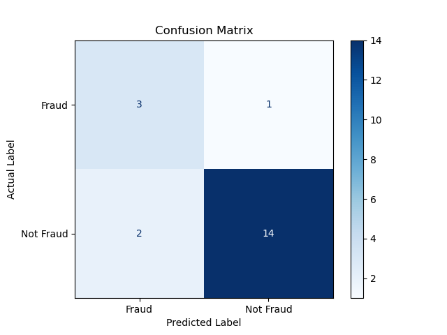
To get precision, recall, F1 score, and other metrics in one step, use the classification_report function on the same arrays:
print(classification_report(actual, predicted, labels=['Fraud', 'Not Fraud'], target_names=['Fraud', 'Not Fraud'])) precision recall f1-score support
Fraud 0.60 0.75 0.67 4
Not Fraud 0.93 0.88 0.90 16
accuracy 0.85 20
macro avg 0.77 0.81 0.78 20
weighted avg 0.87 0.85 0.86 20This prints a clean summary table showing precision, recall, and F1 score for each class, plus overall accuracy. It's one of the quickest ways to evaluate a classification model's performance.
When Accuracy Alone Isn't Enough
Let's revisit our fraud detection dataset with 1,000 transactions: 20 fraudulent and 980 legitimate. What happens if we build the laziest possible model, one that simply predicts "not fraud" for every single transaction?
| Predicted: Fraud | Predicted: Not Fraud | |
|---|---|---|
| Actual: Fraud | 0 (TP) | 20 (FN) |
| Actual: Not Fraud | 0 (FP) | 980 (TN) |
This model's accuracy is 980 / 1,000 = 98.0%. That looks perfectly respectable as a standalone number. But look at the confusion matrix. The model catches exactly zero fraudulent transactions. Its recall is 0%. Every single case of fraud goes undetected. The confusion matrix makes this failure obvious in a way that accuracy alone never could.
Now compare that to our trained model:
| Predicted: Fraud | Predicted: Not Fraud | |
|---|---|---|
| Actual: Fraud | 17 (TP) | 3 (FN) |
| Actual: Not Fraud | 10 (FP) | 970 (TN) |
The trained model has 98.7% accuracy and 85.0% recall. It actually catches fraud. Side by side, the confusion matrices tell a story that a single accuracy number never could.
This is the core problem with classification accuracy as a standalone metric in machine learning, especially with imbalanced data. When one class vastly outnumbers the other, a model can score well on accuracy by simply predicting the majority class every time. The confusion matrix, along with precision, recall, and the F1 score, cuts through that illusion and shows you what's really going on.

Keep Practicing
The best way to solidify your understanding of model evaluation is to build confusion matrices from your own models' predictions. Try adjusting classification thresholds and watch how precision and recall shift in response. That hands-on experimentation is where these concepts really click.
Dataquest's Machine Learning in Python skill path uses confusion matrices across several of its seven courses as you build, evaluate, and optimize classification models on real datasets. The path takes you from supervised machine learning fundamentals through logistic regression, decision trees and random forests, and model optimization.