A Straightforward Guide to Linear Regression in Python
Linear Regression is one of the most basic yet most important models in data science. It helps us understand how we can use mathematics, with the help of a computer, to create predictive models, and it is also one of the most widely used models in analytics in general, from predicting the weather to predicting future profits on the stock market.
In this tutorial, we will define linear regression, identify the tools we need to use to implement it, and explore how to create an actual prediction model in Python including the code details.
Let's get to work.
A Short Introduction to Linear Regression
At its most basic, linear regression means finding the best possible line to fit a group of datapoints that seem to have some kind of linear relationship.
Let's use an example: we work for a car manufacturer, and the market tells us we need to come up with a new, fuel-efficient model. We want to pack as many features and comforts as we can into the new car while making it economic to drive, but each feature we add means more weight added to the car. We want to know how many features we can pack while keeping a low MPG (miles per gallon). We have a dataset that contains information on 398 cars, including the specific information we are analyzing: weight and miles per gallon, and we want to determine if there is a relationship between these two features so we can make better decisions when designing our new model.
If you want to code along, you can download the dataset from Kaggle: Auto-mpg dataset
Let's start by importing our libraries:
import pandas as pd
import matplotlib.pyplot as plt
Now we can load our dataset auto-mpg.csv into a DataFrame called auto, and we can use the pandas head() function to check out the first few lines of our dataset.
auto = pd.read_csv('auto-mpg.csv')
auto.head()| mpg | cylinders | displacement | horsepower | weight | acceleration | model year | origin | car name | |
|---|---|---|---|---|---|---|---|---|---|
| 0 | 18.0 | 8 | 307.0 | 130 | 3504 | 12.0 | 70 | 1 | chevrolet chevelle malibu |
| 1 | 15.0 | 8 | 350.0 | 165 | 3693 | 11.5 | 70 | 1 | buick skylark 320 |
| 2 | 18.0 | 8 | 318.0 | 150 | 3436 | 11.0 | 70 | 1 | plymouth satellite |
| 3 | 16.0 | 8 | 304.0 | 150 | 3433 | 12.0 | 70 | 1 | amc rebel sst |
| 4 | 17.0 | 8 | 302.0 | 140 | 3449 | 10.5 | 70 | 1 | ford torino |
As we can see, there are several interesting features of the cars, but we will simply stick to the two features we are interested in: weight and miles per gallon, or mpg.
We can use matplotlib to create a scatterplot to see the relationship of the data:
plt.figure(figsize=(10,10))
plt.scatter(auto['weight'],auto['mpg'])
plt.title('Miles per Gallon vs. Weight of Car')
plt.xlabel('Weight of Car')
plt.ylabel('Miles per Gallon')
plt.show()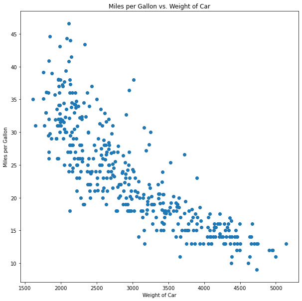
Using this scatterplot, we can easily observe that there does seem to be a clear relationship between the weight of each car and the mpg, where the heavier the car, the fewer miles per gallons it delivers (in short, more weight means more gas).
This is what we call a negative linear relationship, which, simply put, means that as the X-axis increases, the Y-axis decreases.
We can now be sure that if we want to design an economic car, meaning one with high mpg, we need to keep our weight as low as possible. But we want to be as precise as we can. This means we have to determine this relationship as precisely as possible.
Here comes math, and machine learning, to the rescue!
What we really need to determine is the line that best fits the data. In other words, we need a linear algebra equation that will tell us the mpg for a car of X weight. The basic linear algebra formula is as follows:
$ y = xw + b $
This formula means that to find y, we need to multiply x by a certain number, called weight (not to be confused with the weight of the car, which in this case, is our x), plus a certain number called bias (be ready to hear the word "bias" a lot in machine learning with many different meanings).
In this case, our y is the mpg, and our x is the weight of the car.
We could get out our calculators and start testing our math skills until we arrive at a good enough equation that seems to fit our data. For example, we could plug in the following formula into our scatterplot:
$ y = x ÷ -105 + 55 $
And we end up with this line:
plt.figure(figsize=(10,10))
plt.scatter(auto['weight'],auto['mpg'])
plt.plot(auto['weight'], (auto['weight'] / -105) + 55, c='red')
plt.title('Miles per Gallon vs. Weight of Car')
plt.xlabel('Weight of Car')
plt.ylabel('Miles per Gallon')
plt.show()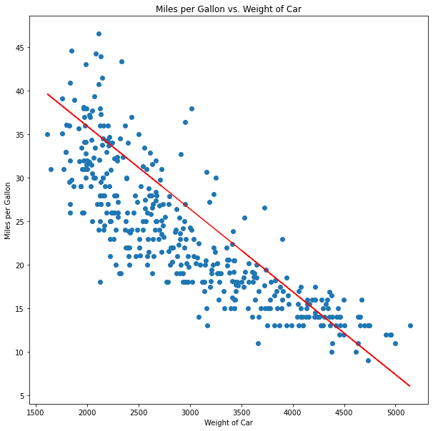
Although this line seems to fit the data, we can easily tell it's off in certain areas, especially around cars that weight between 2,000 and 3,000 pounds.
Trying to determine the best fit Linear Regressionline with some basic calculations and some guesswork is very time-consuming and usually leads us to an answer that tends to be far from the correct one.
The good news is that we have some interesting tools we can use to determine the best fit line, and in this case, we have linear regression.
About SciKit-Learn
scikit-learn, or sklearn for short, is the basic toolbox for anyone doing machine learning in Python. It is a Python library that contains many machine learning tools, from linear regression to random forests — and much more.
We will only be using a couple of these tools in this tutorial, but if you want to learn more about this library, check out the Sci Kit Learn Documentation HERE. You can also check out the Machine Learning Intermediate path at Dataquest
Implementing Linear Regression in Python SKLearn
Let's get to work implementing our linear regression model step by step.
We will be using the basic LinearRegression class from sklearn. This model will take our data and minimize a __Loss Function__ (in this case, one called Sum of Squares) step by step until it finds the best possible line to fit the data. Let's code.
Fist of all, we will need the following libraries:
Pandasto manipulate our data.Matplotlibto plot our data and results.- The
LinearRegressionclass fromsklearn.
Importnat TIP: NEVER import the whole sklearn library; it is massive and will take a long time. Only import the specific tools that you need.
And so, we start by importning our libraries:
import pandas as pd
import numpy as np
import matplotlib.pyplot as plt
from sklearn.linear_model import LinearRegression
Now we load our data into a DataFrame and check out the first few lines (like we did before).
auto = pd.read_csv('auto-mpg.csv')
auto.head()| mpg | cylinders | displacement | horsepower | weight | acceleration | model year | origin | car name | |
|---|---|---|---|---|---|---|---|---|---|
| 0 | 18.0 | 8 | 307.0 | 130 | 3504 | 12.0 | 70 | 1 | chevrolet chevelle malibu |
| 1 | 15.0 | 8 | 350.0 | 165 | 3693 | 11.5 | 70 | 1 | buick skylark 320 |
| 2 | 18.0 | 8 | 318.0 | 150 | 3436 | 11.0 | 70 | 1 | plymouth satellite |
| 3 | 16.0 | 8 | 304.0 | 150 | 3433 | 12.0 | 70 | 1 | amc rebel sst |
| 4 | 17.0 | 8 | 302.0 | 140 | 3449 | 10.5 | 70 | 1 | ford torino |
The next step is to clean our data, but this time, it is ready to be used, we just need to prepare the specific data from the dataset. We create two variables with the necessary data, X for the features we want to use to predict our target and y for the target variable. In this case, we load the weight data form our dataset in X and the mpg data in y.
TIP: When working with only one feature, remember to use double [[]] in pandas so that our series have at least a two-dimensional shape, or you will run into errors when training models.
X = auto[['weight']]
y = auto['mpg']
Since LinearRegression is a class, we need to create a class object where we are going to train our model. Let's call it MPG_Pred (using a capital letter at least at the begining of the variable name is a convention from Python class objects).
There are many specific options you can use to customize the LinearRegression object, take a look at the documentation here. We will stick to the default options for this tutorial.
MPG_Pred = LinearRegression()Now we are ready to train our model using the fit() function with our X and Y variables:
MPG_Pred.fit(X,Y)LinearRegression()And that's it, we have trained our model. But how well do the predictions from our model match the data? Well, we can plot our data to determine how well our predictions, fitted on a line, match the data. This is what we get:
plt.figure(figsize=(10,10))
plt.scatter(auto['weight'], auto['mpg'])
plt.scatter(X,MPG_Pred.predict(X), c='Red')
plt.title('Miles per Gallon vs. Weight of Car')
plt.xlabel('Weight of Car')
plt.ylabel('Miles per Gallon')
plt.show()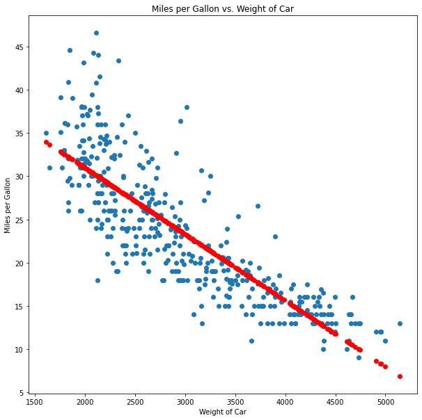
As we can see, our predictions plot (in red) makes a line that seems much better fitted than our original guess, and it was a lot easier than trying to figure it out by hand.
Once again, this is the simplest type of regression, and it has many limitations — for example, it only works on data that has a linear tendency. When we have data that is scattered around a line, like the one in this example, we will only be able to predict approximations of the data, and even when the data follows a linear tendency, but is curved (like this one), we will always get just a straight line, meaning our accuracy will be low.
Nonetheless, it is the basic form of regression and the simplest of all models. Master it, and you can then move on to more complex variations like Multiple Linear Regression (linear regression with two or more features), Polynomial Regression (finds curved lines), Logistic Regression (to use lines to classify data on each side of the line), and (one of my personal favorites) Regression with Stochastic Gradient Descent (our most basic model using one of the most important concepts in Machine Learning: Gradient Descent).
What We Learned
Here are the basic concepts we covered in this tutorial:
- What is linear regression: one of the most basic machine learning models.
- How linear regression works: fitting the best possible line to our data.
- A very brief introduction to the
scikit-learnmachine learning library. - How to implement the
LinearRegressionclass fromsklearn. - An example of linear regression to predict miles per gallon from car weight.
If you want to learn more about Linear Regression and Gradient Descent, check out our Gradient Descent Modeling in Python course, where we go into details about this important concept and how to implement it.