R Markdown Tips, Tricks, and Shortcuts
Turn your data analysis into pretty documents with R Markdown.
R Markdown is an open-source tool for producing reproducible reports in R. It helps you keep all of your code, results, and writing in one place, and format it all in a way that's attractive and digestible.
It's a valuable tool for presenting your data work to others, too. With R Markdown, you have the option to export your work to numerous formats including PDF, Microsoft Word, a slideshow, or an html document for use on a website.
R Markdown is a powerful tool because it can be used for data analysis and data science, to collaborate with others, and communicate results to decision makers.
In this blog post we’ll look at some tips, tricks, and shortcuts for working with R Markdown in RStudio. (If you’d like to learn more about RStudio, check out this Dataquest blog post for RStudio tips and tricks!)
We love using R Markdown for coding in R and authoring content. In fact, we wrote this blog post in R Markdown! Let’s check out some reasons why!
1. Keyboard Shortcuts
Knowing R Markdown keyboard shortcuts will save lots of time when creating reports.
Here are some of the essential R Markdown shortcuts:
- Insert a new code chuck with
Command + Option + Ion a Mac, orCtrl + Alt + Ion Linux and Windows. - Output your document in the format specified in your YAML header with
Command + Shift + Kon a Mac, orCtrl + Shift + Kon Linux and Windows. The “k” is short for “knit”!
Next we’ll cover shortcuts to run code chunks. But before doing this it is often a good idea to restart your R session and start with a clean environment. Do this with Command + Shift + F10 on a Mac or Ctrl + Shift + F10 on Linux and Windows.
- Run all chunks above the current chunk with
Command + Option + Pon a Mac;Ctrl + Alt + Pon Linux and Windows. - Run the current chunk with
Command + Option + CorCommand + Shift + Enteron a Mac;Ctrl + Alt + CorCtrl + Shift + Enteron Linux and Windows. - Run the next chunk with
Command + Option + Non a Mac;Ctrl + Alt + Non Linux and Windows. - Run all chunks with
Command + Option + RorCommand + A + Enteron a Mac;Ctrl + Alt + RorCtrl + A + Enteron Linux and Windows.
2. Quickly Preview Your Document
R Markdown provides many format options for compiling your document. But rendering your work as a PDF or a presentation can take much longer than compiling to HTML. For this reason, it is generally useful to output your document to HTML while authoring because this enables to iterate quickly.
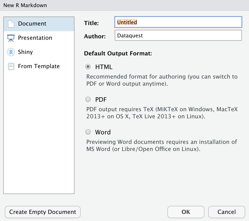
When you open a new R Markdown file, the default output format is HTML — when you compile your report, you can easily view it in a web browser. This default setting can save you time! When you near a finished product, you change the output to the format of your choosing and make the final touches then.
3. Know Your Code Chunk Options
One of the great things about R Markdown is that you have many options for controlling how each chunk of code is evaluated and presented. This allows you to build presentations and reports from the ground up, including code, plots, tables, and images, while only presenting the essential information to the intended audience. For example, you can include a plot of your results without showing the code used to generate it.
Mastering these code chunk options is essential to becoming a proficient R Markdown user:
echo = FALSE: Hide the code, but run code and produce all outputs, plots, warnings and messages.eval = FALSE: Show code, but do not evaluate it.- fig.show = "hide": Hides plots.
include = FALSE: Runs code, but suppresses all output. This is helpful for setup code. You can see an example of this in the first code chunk when you open a new R Markdown document!message = FALSE: Prevent packages from printing messages when they load. This also suppress messages generated by functions.results = "hide": Hides printed output.warning = FALSE: Prevents packages and functions from displaying warnings.
4. Use Inline Code
Directly embed R code into an R Markdown document with inline code. This is useful when you want to include information about your data in the written summary.
Use inline code with r and add the code to evaluate within the backticks. For example, we used inline code when writing this blog post to automatically number each section, so that we didn’t have to manually add them ourselves. So how did we do it? We started by creating a variable called tip_number and in the setup code chunk, and set the value to zero, like this:
tip_number <- 0Then we added the following inline code to each section to grow the number by one at each iteration:
r paste0(tip_number <- tip_number + 1, ". ")Hey, wait a minute! How did we include that last line of code in this blog post authored in R Markdown without messing up the section numbering below? With code chunk options! The code example above is written in a code chunk with the option eval = FALSE to prevent the code from running. Like this:

As you can see, R Markdown is a powerful tool because it gives you a lot of control over the output of your document!
5. Use TinyTex
With R Markdown you can use the LaTeX document preparation system to output high-quality reports. LaTeX is especially useful when reports include scientific or mathematical symbols and notation. For example, we use LaTeX here at Dataquest for authoring statistics content that uses mathematical notation.
But LaTeX distributions such as TeX Live, MiKTeX, and MacTeX, require about 5 gigabytes of disk space on your hard drive! In contrast, TinyTex uses only about 150 megabytes when it’s installed.
Install TinyTex with install.packages('tinytex') or tinytex::install_tinytex(). Uninstall TinyTex with tinytex::uninstall_tinytex().
With TinyTex installed, there is nothing else you need to do to output a PDF document if you’ve specified PDF as the output format!
To compile a LaTeX document to PDF, call one of these tinytex functions: pdflatex(), xelatex(), and lualatex(). The function to use depends on the LaTeX engine that you want to use.
TinyTex developer and R Markdown superstar Yihui Xie says that’s about all the average R user needs to know about TinyTex. Why? Because the LaTeX functions mentioned will automatically detect and install any missing LaTeX packages that are required!
6. Generate an R Markdown Document with an R Script
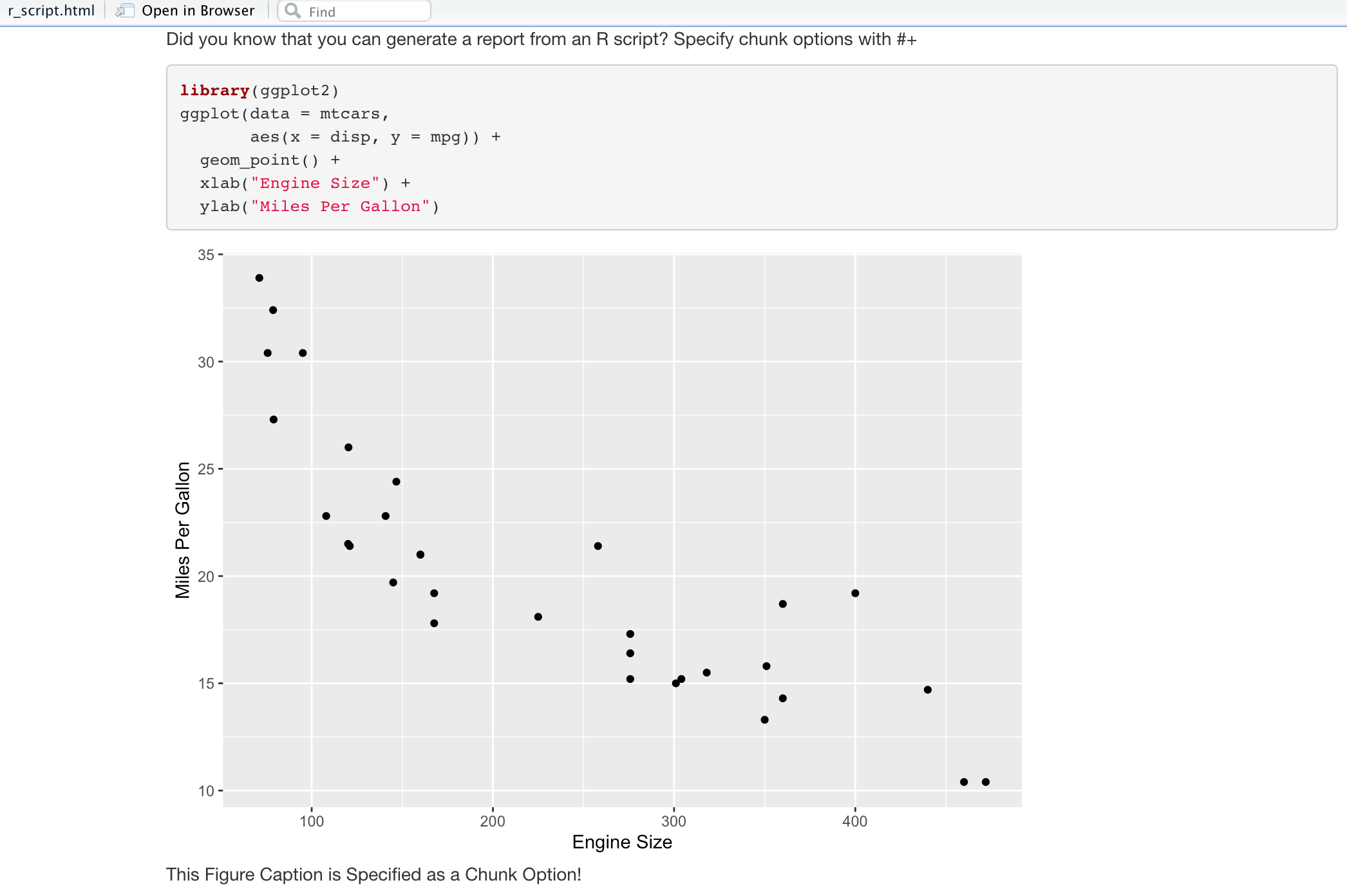
Did you know that you can generate an R Markdown document from an R Script? To do this, capture commentary with #'. You can even specify code chunk options with #+. Here’s an example:

This R script is saved with the file name “r_script.R”. To render this document as an R Markdown document, we specify the spin() function from knitr, like this:
knitr::spin("r_script.R", knit = FALSE, format = "Rmd")
This generates an R Markdown document that looks like this:

And when you knit this document, this HTML output is returned:
7. Generate an R Script with an R Markdown Document
You may be wondering if there’s a way to convert an R Markdown document to an R Script? There is! The knitr package also offers a function for that, called purl(). Here’s the command to convert our R Markdown document back to an R script:
knitr::purl("r_script.Rmd", documentation = 2)
Note that you must specify documentation = 2 to return full documentation in #' comments. If your document is pure code, specify documentation = 0.
8. Add Line Breaks in R Markdown
How difficult can it be to add a line break in your output? It’s not. But figuring this out can be a bit tricky!
To break a line in R Markdown and have it appear in your output, use two trailing spaces and then hit return. Let’s look at an example.
Here, we did not specify two trailing spaces between the two sentences in the first (top) group. But we did specify two trailing spaces between the two sentences in the second (bottom) group.

The result after we knitted the document? Check it out!

9. Add Blank Lines in R Markdown
Because we just covered line breaks, let’s also discuss how to add empty lines to your document. This can be useful when you want to add white space to reduce clutter in your document.
To have one or many empty lines appear in your output, specify <br>. Let’s look at an example.
Here, we did not specify two <br> commands between the two sentences in the first (top) group. But we did specify two <br> commands between the two sentences in the second (bottom) group.

And here’s the result!

10. Query SQL in R Markdown
You can query SQL in R Markdown by creating a {sql} code chunk.
You’ll start by generating an in-memory SQL database to use in this example. You’ll generate a SQL database of the well-known “mtcars” dataset. Here’s the code:

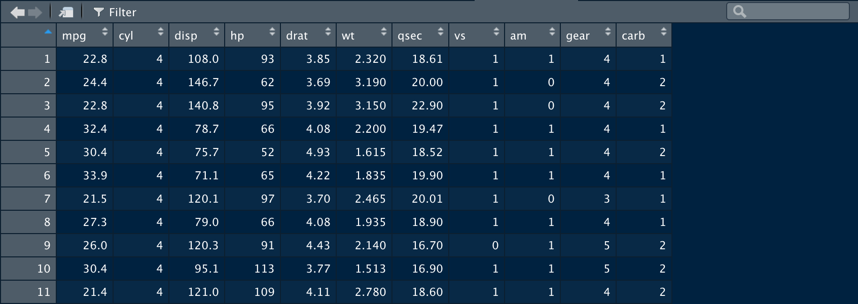
In a new code chunk, write a SQL query to select all cars from the database with a four-cylinder engine. Be sure to change the type of this chunk to {sql}. This command returns a dataframe that you’ll save as mt_cars_df:

Specify output.var = "mt_cars_df" to save the results of your query to a dataframe. The dataframe looks like this:
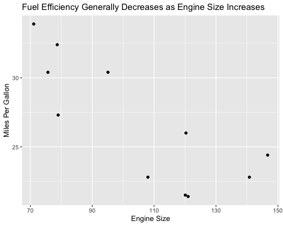
You can use this dataframe in R code chunks to perform analysis or to generate a ggplot, for example:

11. Use Chunk Names
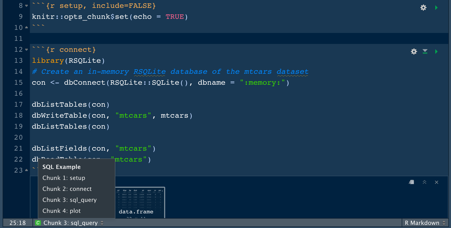
Naming code chunks can be useful for long documents with many chunks. With R code chunks, for example, name the chunk like this: {r my_boring_chunk_name}.
With named code chunks, you can navigate between chunks in the code chunk navigator included at the bottom of the R Markdown window pane. This can also make plots easy to identify by name so they can be used in other sections of your document.
We’ve added chunk names to the SQL example from above. Here’s what we see in the navigator:
12. Take it to the Cloud!
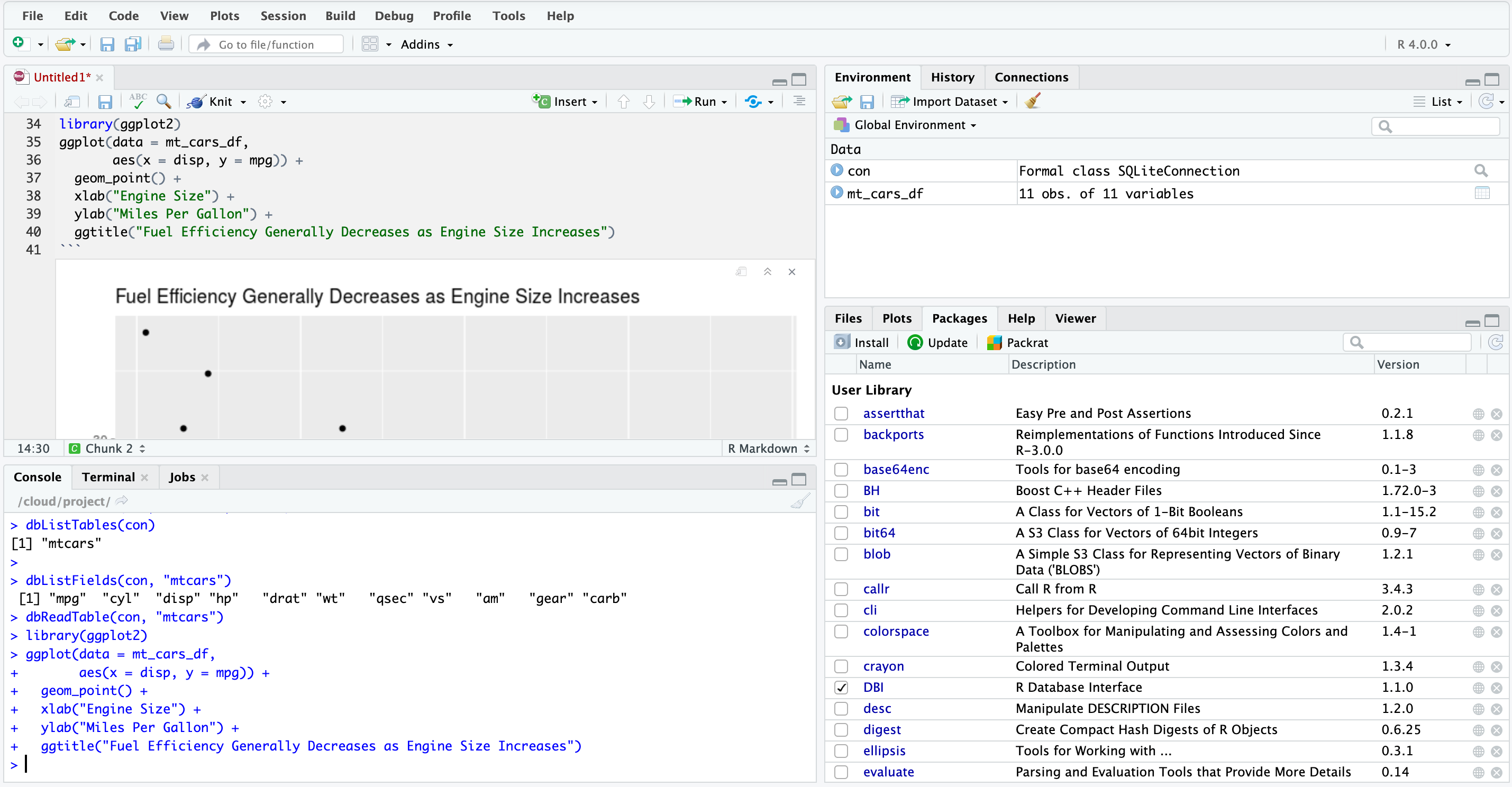
RStudio now offers a cloud-based version of RStudio Desktop called RStudio Cloud. RStudio Cloud allows you to author in R Markdown without installing software, you only need a web browser.
Work in RStudio Cloud is organized into projects similar to the desktop version, but RStudio Cloud enables you to specify the version of R you wish to use for each project.
RStudio Cloud also makes it easy and secure to share projects with colleagues, and ensures that the working environment is fully reproducible every time the project is accessed. This is great for writing reproducible reports in R Markdown!
As you can see, the layout of RStudio Cloud is very similar to authoring an R Markdown document in RStudio Desktop:
Bonus: R Markdown Cheatsheet
RStudio has published numerous cheatsheets for working with R, including a detailed cheatsheet on using R Markdown! The R Markdown cheatsheet can be accessed from within RStudio by selecting Help > Cheatsheets > R Markdown Cheat Sheet.
Additional Resources
RStudio has published a few in-depth how to articles about using R Markdown. Find them here.
To learn more about RStudio, check out 23 RStudio Tips, Tricks, and Shortcuts
The R Markdown Cookbook is a comprehensive, free online book that countains almost everything you need to know about R Markdown.