Getting Started with R Markdown — Guide and Cheatsheet
Turn your data analysis into pretty documents with R Markdown.
In this blog post, we’ll look at how to use R Markdown. By the end, you’ll have the skills you need to produce a document or presentation using R Markdown, from scratch!
We’ll show you how to convert the default R Markdown document into a useful reference guide of your own. We encourage you to follow along by building out your own R Markdown guide, but if you prefer to just read along, that works, too!
R Markdown is an open-source tool for producing reproducible reports in R. It enables you to keep all of your code, results, plots, and writing in one place. R Markdown is particularly useful when you are producing a document for an audience that is interested in the results from your analysis, but not your code.
R Markdown is powerful because it can be used for data analysis and data science, collaborating with others, and communicating results to decision makers. With R Markdown, you have the option to export your work to numerous formats including PDF, Microsoft Word, a slideshow, or an HTML document for use in a website.
We’ll use the RStudio integrated development environment (IDE) to produce our R Markdown reference guide. If you’d like to learn more about RStudio, check out our list of 23 awesome RStudio tips and tricks!
Here at Dataquest, we love using R Markdown for coding in R and authoring content. In fact, we wrote this blog post in R Markdown! Also, learners on the Dataquest platform use R Markdown for completing their R projects.
We included fully-reproducible code examples in this blog post. When you’ve mastered the content in this post, check out our other blog post on R Markdown tips, tricks, and shortcuts.
Okay, let’s get started with building our very own R Markdown reference document!
R Markdown Guide and Cheatsheet: Quick Navigation
- 1. Install R Markdown
- 2. Default Output Format
- 3. R Markdown Document Format
- 4. Section Headers
- 5. Bulleted and Numbered Lists
- 6. Text Formatting
- 7. Links
- 8. Code Chunks
- 9. Running Code
- 10. Control Behavior with Code Chunk Options
- 11. Inline Code
- 12. Navigating Sections and Code Chunks
- 13. Table Formatting
- 14. Output Format Options
- 15. Presentations
- 16. Add a Table of Contents
- 17. Reproducible Reports with RStudio Cloud
- More R Markdown Tips, Tricks, and Shortcuts
- Bonus: R Markdown Cheatsheet
- Additional Resources
1. Install R Markdown
R Markdown is a free, open source tool that is installed like any other R package. Use the following command to install R Markdown:
install.packages("rmarkdown")Now that R Markdown is installed, open a new R Markdown file in RStudio by navigating to File > New File > R Markdown…. R Markdown files have the file extension “.Rmd”.
2. Default Output Format
When you open a new R Markdown file in RStudio, a pop-up window appears that prompts you to select output format to use for the document.
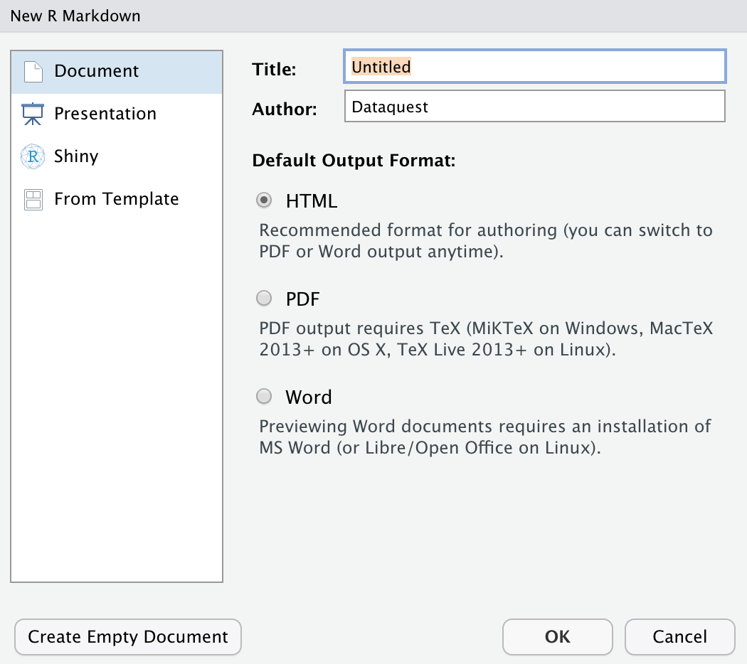
The default output format is HTML. With HTML, you can easily view it in a web browser.
We recommend selecting the default HTML setting for now — it can save you time! Why? Because compiling an HTML document is generally faster than generating a PDF or other format. When you near a finished product, you change the output to the format of your choosing and then make the final touches.
One final thing to note is that the title you give your document in the pop-up above is not the file name! Navigate to File > Save As.. to name, and save, the document.
3. R Markdown Document Format
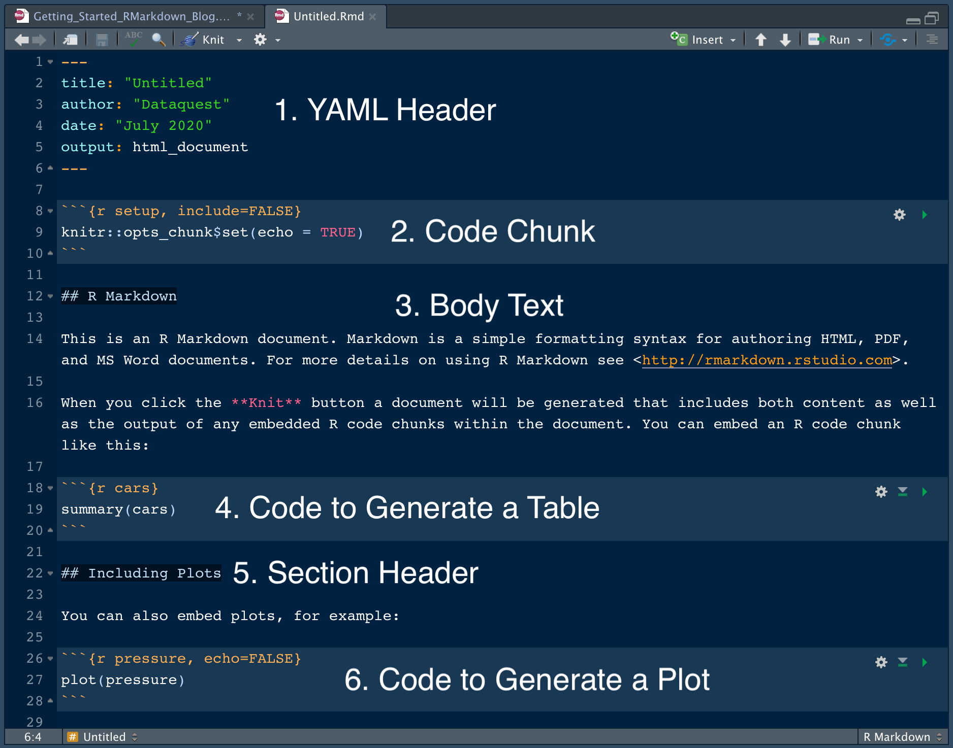
Once you’ve selected the desired output format, an R Markdown document appears in your RStudio pane. But unlike an R script which is blank, this .Rmd document includes some formatting that might seem strange at first. Let’s break it down.
We’ve highlighted six different sections of this R Markdown document to understand what is going on:
- YAML Header: Controls certain output settings that apply to the entire document.
- Code Chunk: Includes code to run, and code-related options.
- Body Text: For communicating results and findings to the targeted audience.
- Code to Generate a Table: Outputs a table with minimal formatting like you would see in the console.
- Section Header: Specified with ##.
- Code to Generate a Plot: Outputs a plot. Here, the code used to generate the plot will not be included because the parameter echo=FALSE is specified. This is a chunk option. We’ll cover chunk options soon!
This document is ready to output as-is. Let’s “knit,” or output, the document to see how these formatting specifications look in a rendered document. We do this in RStudio by clicking the knit button. Knitting the document generates an HTML document, because that’s the output format we’ve specified.
The shortcut to knit a document is Command + Shift + K on a Mac, or Ctrl + Shift + K on Linux and Windows. The “k” is short for “knit”!
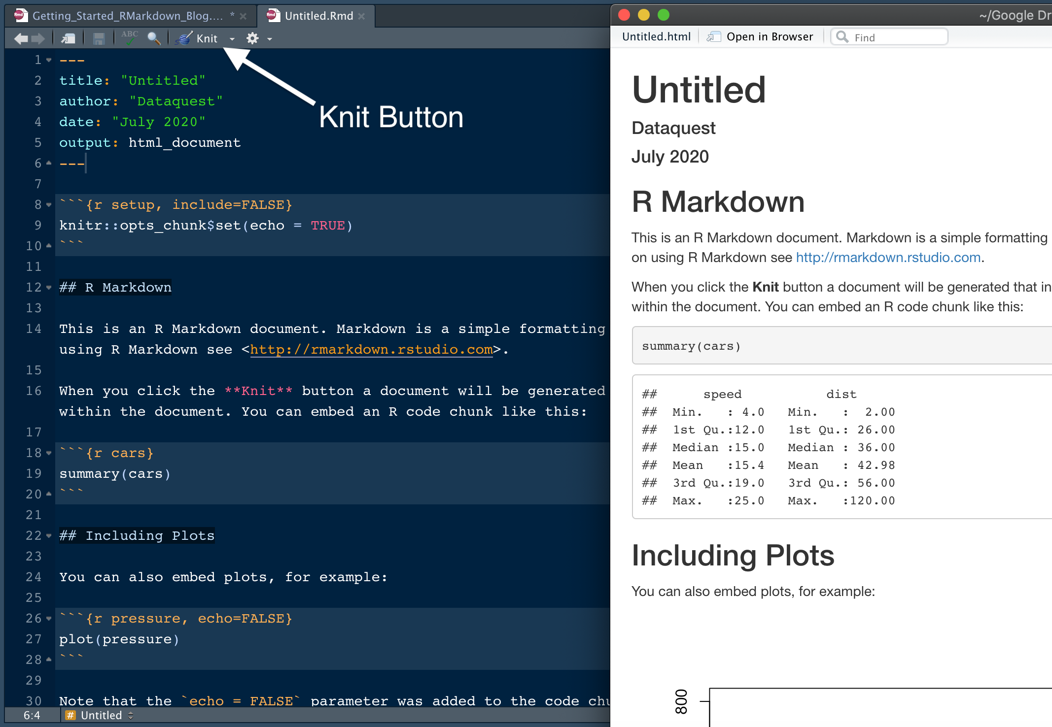
The image above illustrates how the R Markdown document, on the left, looks when it’s output to HTML, on the right.
Notice that the default .Rmd file in RStudio includes useful guidance on formatting R Markdown documents. We’ll save this document as RMarkdown_Guide.Rmd so we can add to it as we progress through this tutorial. We gave the document the title “R Markdown Guide” in the YAML header. We encourage you to do the same so you can build your very own R Markdown reference guide!
Note: If you are working in R Markdown outside of RStudio, use the function rmarkdown::render() to compile your document. Provide the name of your document in quotes as the function argument. For example:
rmarkdown::render("RMarkdown_Guide.Rmd")4. Section Headers
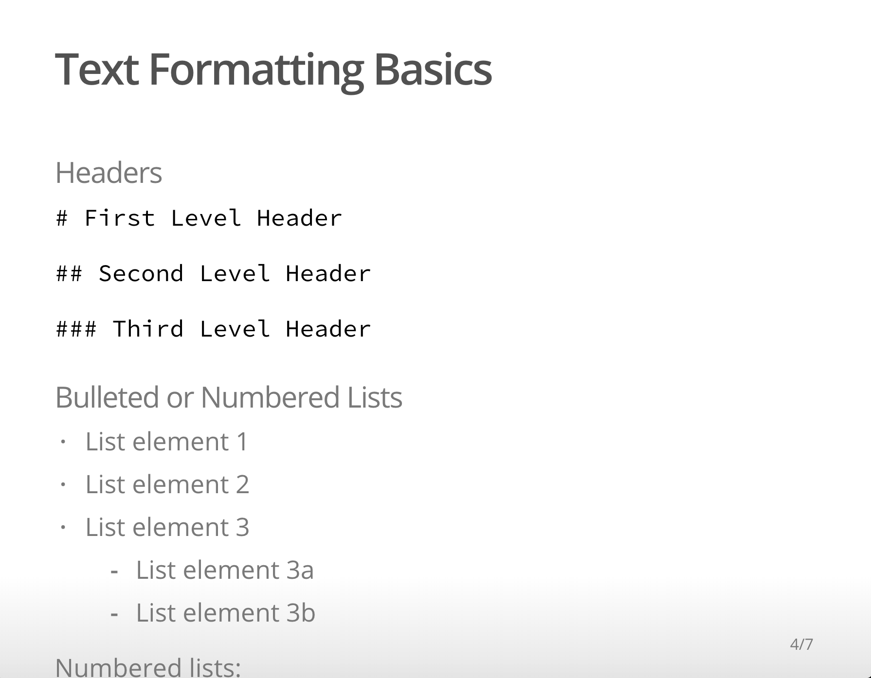
Next, we’ll cover the fundamentals of text formatting in an .Rmd file. An R Markdown file is a plain-text file written in Markdown, which is a formatting syntax. We begin with section headers.
Notice in the default .Rmd file that there are two sections in the document, R Markdown and Including Plots. These are second-level headers, because of the double hash marks (##). Let’s create a new second-level header in our Guide called Text Formatting Basics by entering:
## Text Formatting BasicsFollow this with a third-level header, called Headers, like this:
## Text Formatting Basics
### Headers
We’ll build-out our Guide with syntax requirements for first, second, and third-level headers. We want our Guide to show the code to generate headers.
So, to add the formatting requirements for headers to our Guide, we add the following:
# First Level Header
## Second Level Header
### Third Level Header
Tip: Insert a blank line between each line of code to separate them at output. And always have at least one blank line in between format elements that are adjacent, but different from each other, such as section headers and body text.
The .Rmd document and the output looks like this:
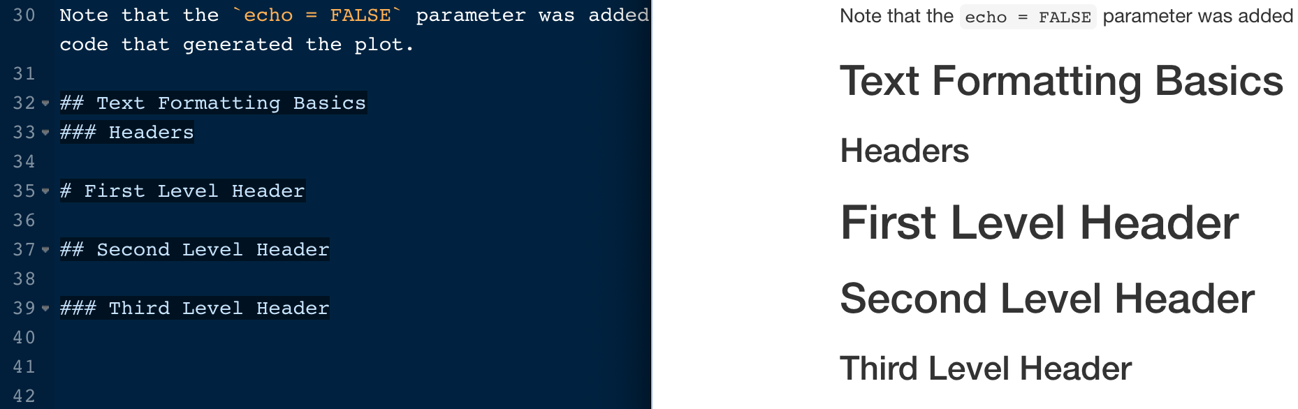
In the image above, we see how second- and third-level headers look when rendered. We also specified the syntax for creating headers with #, ## or ###. This is a great example of how simple, yet powerful, formatting in R Markdown can be.
If you don’t want the headers to render as headers in the final output, wrap the code in backticks like this, to format the text as code:
# First Level Header5. Bulleted and Numbered Lists
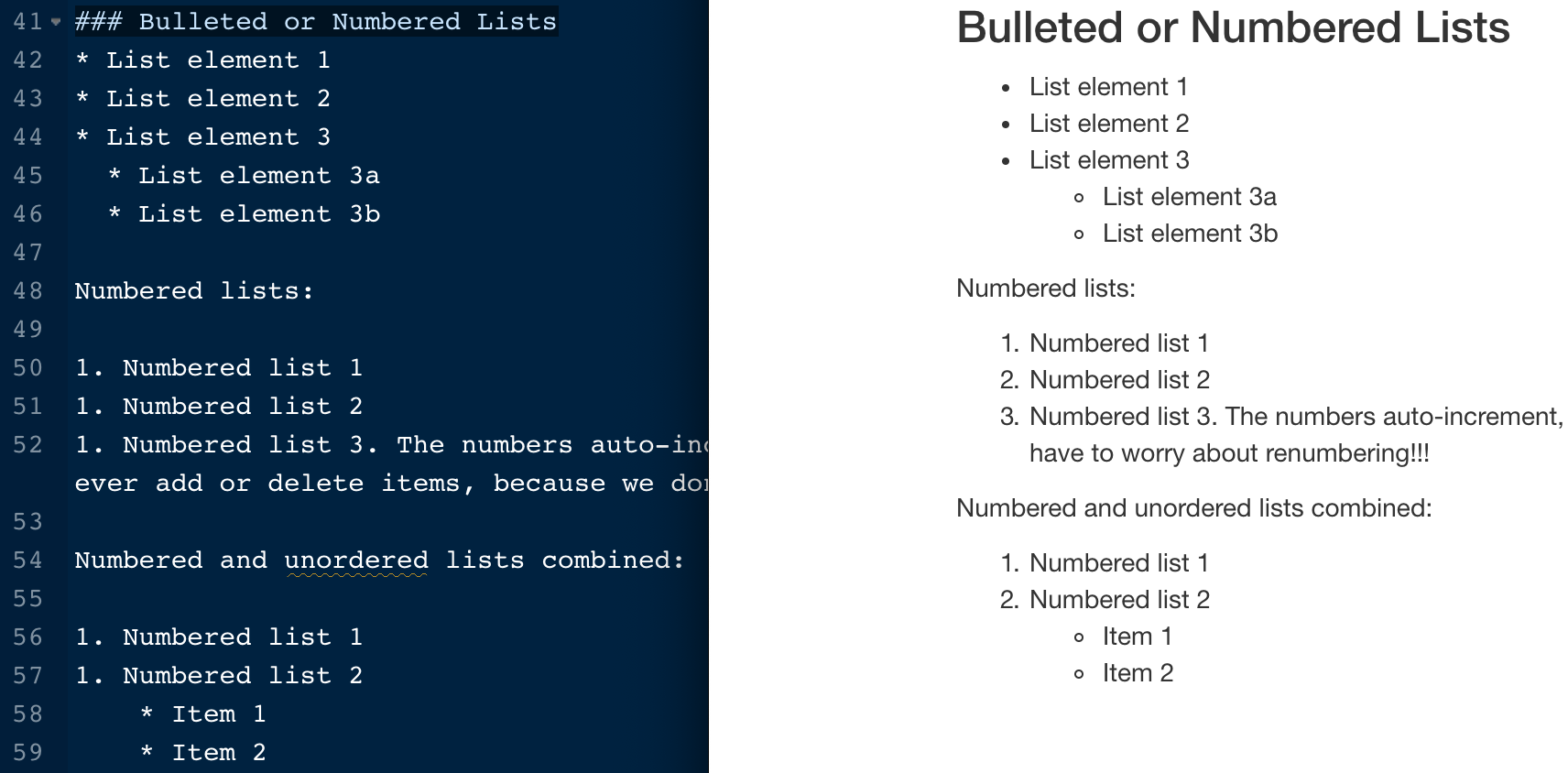
Now we’ll create a new third-level header called Bulleted and Numbered Lists and type the following into the Guide to generate unordered lists:
* List element 1
* List element 2
* List element 3
 * List item 3a
 * List item 3b
In fact, the characters *, - and + all work for generating unordered list items.
Here is the syntax required for numbered lists:
1. Numbered list 1
1. Numbered list 2
1. Numbered list 3.
The numbers auto-increment, so we only need to enter “1.”. This is great if we ever add or delete items, because we don’t have to worry about renumbering!
It’s also possible to combine numbered and unordered lists. Hit tab twice to indent the unordered bullets:
1. Numbered list 1
1. Numbered list 2
 * Item 1
 * Item 2
Here’s a side-by-side view of how this formatting looks in our Guide and our output:
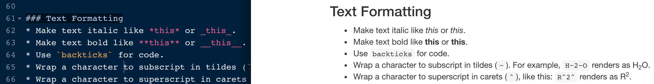
6. Text Formatting
We’ll continue building out our R Markdown Guide by adding basic text formatting. Create a new third-level header called Text Formatting and copy or type, the following:
* Make text italic like *this* or _this_.
* Make text bold like **this** or __this__.
* Use backticks for code.
* Wrap a character to subscript in tildes (~). For example, H~2~O renders as H~2~O.
* Wrap a character to superscript in carets (^), like this: R^2^ renders as R^2^.
Here’s how this looks when rendered:
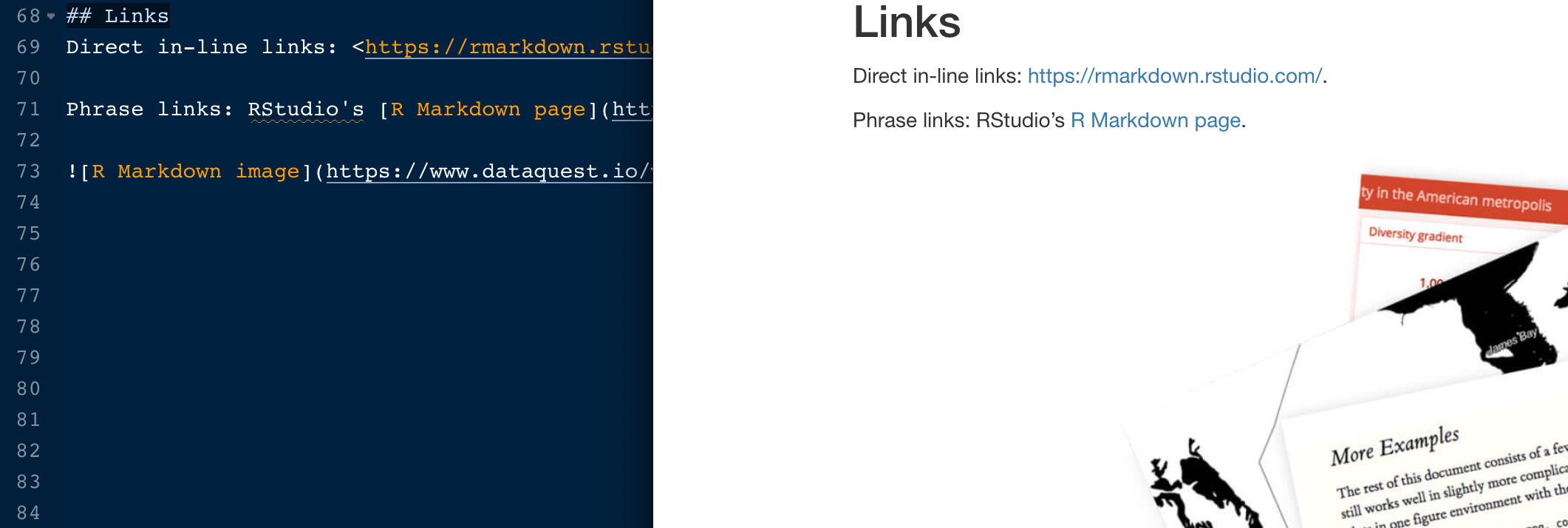
7. Links
R Markdown makes it easy to link to websites and images. In this section of our Guide called Links, we document the following:
Direct in-line links: <https://rmarkdown.rstudio.com/>.
Phrase links: RStudio's [R Markdown page](https://rmarkdown.rstudio.com/).
And here’s the HTML output:
8. Code Chunks
To run blocks of code in R Markdown, use code chunks. Insert a new code chunk with:
Command + Option + Ion a Mac, orCtrl + Alt + Ion Linux and Windows.- Another option is the “Insert” drop-down Icon in the toolbar and selecting R.
We recommend learning the shortcut to save time! We’ll insert a new code chunk in our R Markdown Guide in a moment.
9. Running Code
RStudio provides many options for running code chunks in the “Run” drop-down tab on the toolbar:
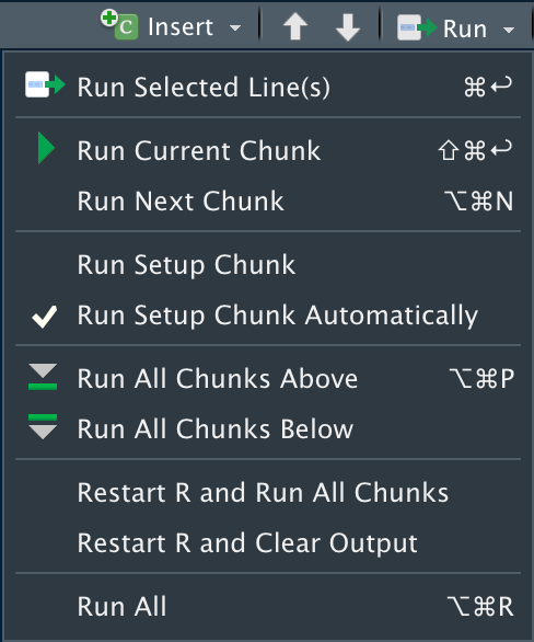
Before running code chunks it is often a good idea to restart your R session and start with a clean environment. Do this with Command + Shift + F10 on a Mac or Control + Shift + F10 on Linux and Windows.
To save time, it’s worth learning these shortcuts to run code:
- Run all chunks above the current chunk with
Command + Option + Pon a Mac, orCtrl + Alt + Pon Linux and Windows. - Run the current chunk with
Command + Option + CorCommand + Shift + Enteron a Mac. On Linux and Windows, useCtrl + Alt + CorCtrl + Shift + Enterto run the current chunk. - Run the next chunk with
Command + Option + Non a Mac, orCtrl + Alt + Non Linux and Windows. - Run all chunks with
Command + Option + RorCommand + A + Enteron a Mac. On Linux and Windows, useCtrl + Alt + RorCtrl + A + Enterto run all chunks.
> install.packages("Dataquest")
Start learning R today with our Introduction to R course — no credit card required!
10. Control Behavior with Code Chunk Options
One of the great things about R Markdown is that you have many options to control how each chunk of code is evaluated and presented. This allows you to build presentations and reports from the ground up — including code, plots, tables, and images — while only presenting the essential information to the intended audience. For example, you can include a plot of your results without showing the code used to generate it.
Mastering code chunk options is essential to becoming a proficient R Markdown user. The best way to learn chunk options is to try them as you need them in your reports, so don’t worry about memorizing all of this now. Here are the key chunk options to learn:
echo = FALSE: Do not show code in the output, but run code and produce all outputs, plots, warnings and messages. The code chunk to generate a plot in the image below is an example of this.eval = FALSE: Show code, but do not evaluate it.fig.show = "hide": Hide plots.include = FALSE: Run code, but suppress all output. This is helpful for setup code. You can see an example of this in the top code chunk of the image below.message = FALSE: Prevent packages from printing messages when they load. This also suppress messages generated by functions.results = "hide": Hides printed output.warning = FALSE: Prevents packages and functions from displaying warnings.
11. Inline Code
Directly embed R code into an R Markdown document with inline code. This is useful when you want to include information about your data in the written summary. We’ll add a few examples of inline code to our R Markdown Guide to illustrate how it works.
Use inline code with r and add the code to evaluate within the backticks. For example, here’s how we can summarize the number of rows and the number of columns in the cars dataset that’s built-in to R:
## Inline Code

The cars dataset contains r nrow(cars) rows and r ncol(cars) columns.
Here’s the side-by-side view comparing how this looks in R Markdown and in the HTML output:

The example above highlights how it’s possible to reduce errors in reports by summarizing information programmatically. If we alter the dataset and change the number of rows and columns, we only need to rerun the code for an accurate result. This is much better than trying to remember where in the document we need to update the results, determining the new numbers, and manually changing the results. R Markdown is a powerful because it can save time and improve the quality and accuracy of reports.
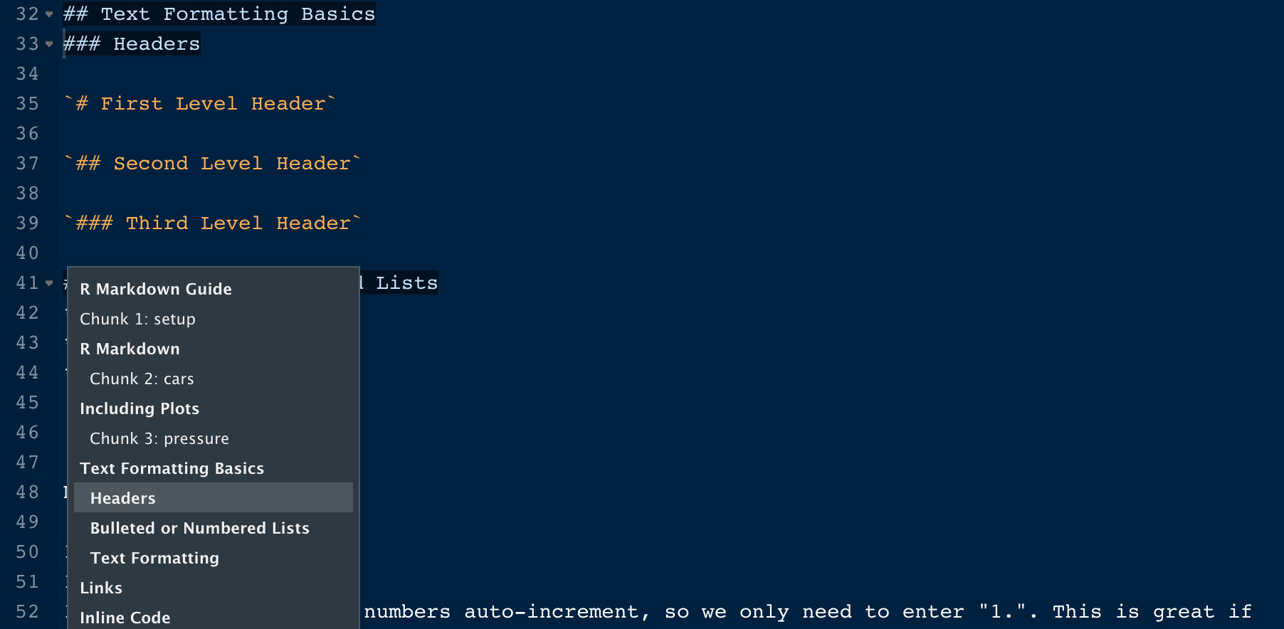
12. Navigating Sections and Code Chunks
Naming code chunks is useful for long documents with many chunks. With R code chunks, name the chunk like this: {r my_boring_chunk_name}.
With named code chunks, you can navigate between chunks in the navigator included at the bottom of the R Markdown window pane. This can also make plots easy to identify by name so they can be used in other sections of your document. This navigator is also useful for quickly jumping to another section of your document.
Here’s what we see in the navigator for our R Markdown Guide:
13. Table Formatting
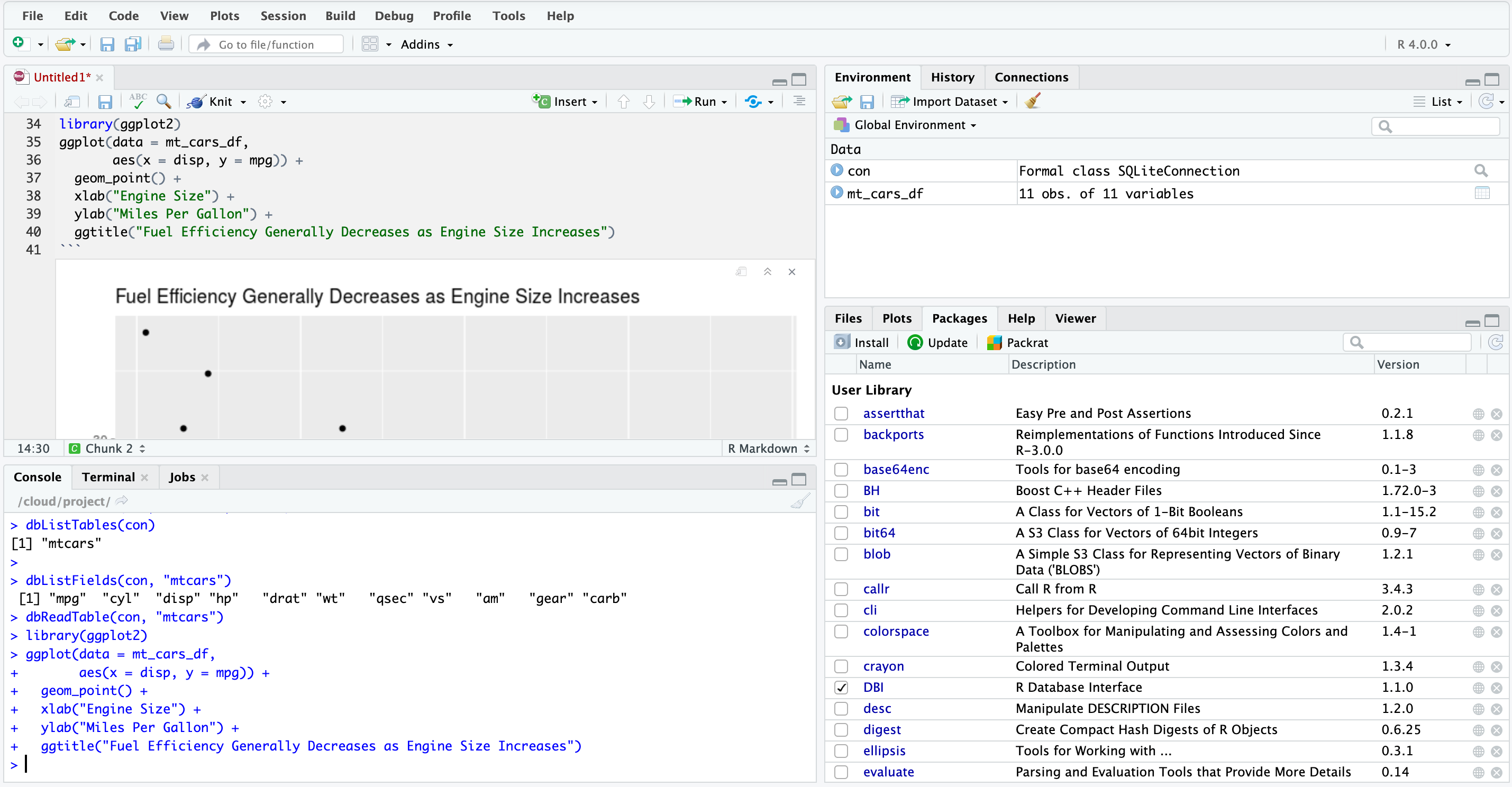
As mentioned earlier in this post, tables in R Markdown are displayed as you see them in the R console by default. To improve the aesthetics of a table in an R Markdown document, use the function knitr::kable(). Here’s an example:
knitr::kable(head(cars), caption = "The First Few Rows of the Cars Dataset")Here’s how this looks in our Guide, and when rendered:
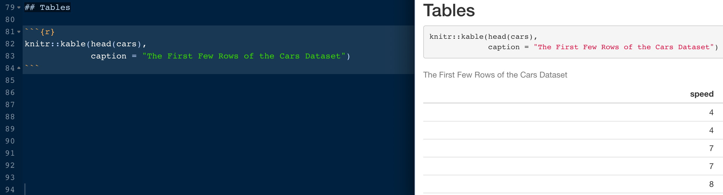
There are many other packages for creating tables in R Markdown.
A word of caution: Formatting tables can be very time-consuming. We recommend sticking to the basics at first when learning R Markdown. As your skills grow, and table formatting needs become apparent, consult other packages as needed.
14. Output Format Options
Now that we have a solid understanding about how to format an R Markdown document, let’s discuss format options. Format options that apply to the entire document are specified in the YAML header. R Markdown supports many types of output formats.
The metadata specified in the YAML header controls the output. A single R Markdown document can support many output formats. Recall that rendering to HTML is generally faster than PDF. If you want to preview your document in HTML but will eventually output your document as a PDF, comment-out the PDF specifications until they are needed, like this:
---
title: "R Markdown Guide"
author: "Dataquest"
date: "7/8/2020"
output: html_document
# output: pdf_document
# output: ioslides_presentation
---
As you can see here, we’ve also included the metadata we need to output our R Markdown Guide as a presentation.
15. Presentations
The rmarkdown package supports four types of presentations. Other R packages are available, such as revealjs, that expand the capabilities of R Markdown. We’ll briefly outline the presentation formats that are built-into R Markdown, and then we’ll look at an example.
The four presentation options and the format they output to are:
- beamer_presentation: PDF
- ioslides_presentation: HTML
- powerpoint_presentation: Microsoft Powerpoint
- slidy_presentation: HTML
Let’s convert our R Markdown Guide to an ioslides presentation. The ioslides option compiles to HTML which is useful for delivering presentations during remote meetings with screen sharing, for example. We convert our Guide to an ioslides presentation with output: ioslides_presentation.
---
title: "R Markdown Guide"
author: "Dataquest"
date: "7/8/2020"
# output: html_document
# output: pdf_document
output: ioslides_presentation
---
Note that we “commented-out” the HTML and PDF format options so that they are ignored when compiling the document. This is a handy technique for keeping other output options available.
When we knit, the R Markdown Guide and HTML presentation appears with each second-level header marking the beginning of a new slide. This works well except for our section “Text Formatting Basics” which has a few third-level header sections:
To address this situation with manual line breaks, we insert *** as needed before each third-level header, like this:
## Text Formatting Basics
### Headers# First Level Header## Second Level Header### Third Level Header***
### Bulleted or Numbered Lists
* List element 1
* List element 2
* List element 3
 * List element 3a
 * List element 3b
This will move “Bulleted or Numbered Lists” to its own slide:
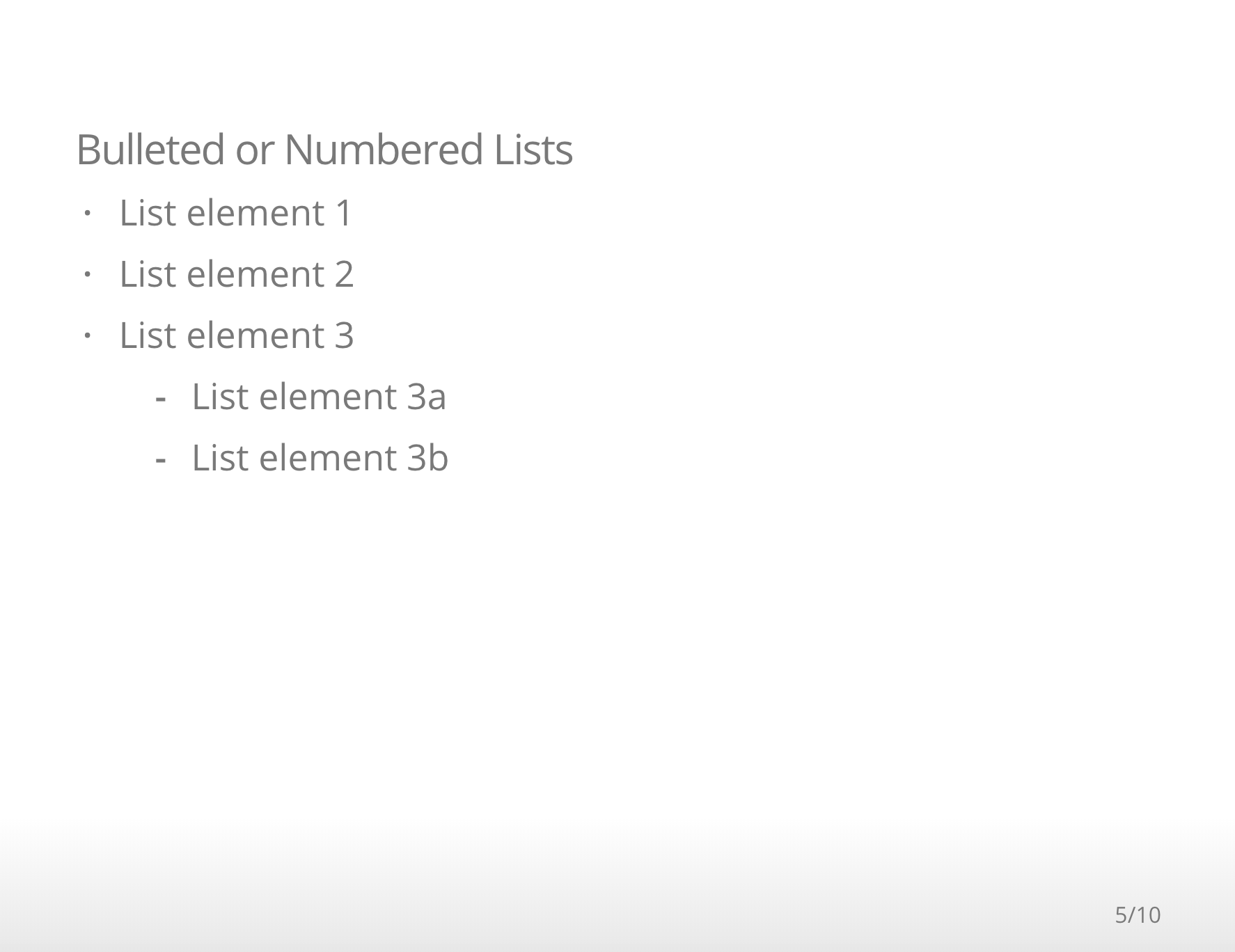
Consult the links above for each presentation format to see the options available to customize the presentation appearance.
16. Add a Table of Contents
You’ll notice that this blog post includes a table of contents. You may recall we wrote this blog post in R Markdown. We added the table of contents to this blog post with one line of code in the YAML header, toc: true. This is how it looks:
output:
 html_document:
    toc: true
Notice the indentation used at each level, and don’t forget to add the : after html_document!
17. Reproducible Reports with RStudio Cloud
Everything you learned here can be applied on a cloud-based version of RStudio Desktop called RStudio Cloud. RStudio Cloud enables you to produce reports and presentations R Markdown without installing software, you only need a web browser.
Work in RStudio Cloud is organized into projects similar to the desktop version, but RStudio Cloud enables you to specify the version of R you wish to use for each project.
RStudio Cloud also makes it easy and secure to share projects with colleagues, and ensures that the working environment is fully reproducible every time the project is accessed. This is especially useful for writing reproducible reports in R Markdown!
As you can see, the layout of RStudio Cloud is very similar to authoring an R Markdown document in RStudio Desktop:
Using R Markdown in RStudio Cloud requires certain packages. When you open a new R Markdown document in RStudio Cloud for the first time, the program provides a prompt asking if you would like to installed the required packages:
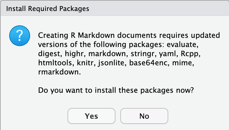
Once the packages are installed you’ll be ready to create and knit R Markdown documents right away!
Bonus: R Markdown Cheatsheet
RStudio has published numerous cheatsheets for working with R, including a detailed cheatsheet on using R Markdown! The R Markdown cheatsheet can be accessed from within RStudio by selecting Help > Cheatsheets > R Markdown Cheat Sheet.
Additional Resources
To learn more about R Markdown, check out R Markdown Tips, Tricks, and Shortcuts
To learn more about RStudio, check out 23 RStudio Tips, Tricks, and Shortcuts
RStudio has published a few in-depth how to articles about using R Markdown. Find them here.
The R Markdown Cookbook is a comprehensive, free online book that contains almost everything you need to know about R Markdown.
Hadley Wickham provides a great overview of authoring with R Markdown in the book R for Data Science.
Check out this R Markdown authoring quick tour, and this comprehensive online lesson from RStudio.
RStudio has also published this useful R Markdown reference guide.
R Markdown understands Pandoc’s Markdown, a version of Markdown with more features. This Pandoc guide provides and extensive resource for formatting options.