R Functions Tutorial: Writing, Scoping, Vectorizing, and More!
When we're programming in R, we often want to take a data set, or some subsection of a data set, and do something to it. This is the kind of task that might be very time-consuming if we were working in a spreadsheet. But in R, we can perform very complex operations on large data sets quite quickly using functions.
What are R functions? In this tutorial, we're going to take a close look at some different types of functions in R, how they work, and why they're useful for data science and data analysis tasks.
R Functions: Inputs and Outputs
In programming, a function describes some process that takes some input, performs some operation or operations on it, and returns the resulting output.
You may recall this concept from math classes, where you probably learned the squaring function, which takes an input number and multiples that number by itself to produce the output answer.
In R, functions do the same thing: they take inputs and run some R code to produce and return an output. If you’ve run any R code before, you’ve probably used built-in R functions like print() or summary(). These functions take in an input, called an argument in programming, and perform actions on it to produce an output.
We'll start our exploration of functions by loading a cool data set from Kaggle that contains almost 7,000 US Data Science Job postings. Imagine that we wanted to do some data analysis with this data set to learn more about data science job postings. One of the first things we might want to do is take a look at the data we've imported, and the summary() function is perfect for that.
This function and the similar head() function are really useful in data science work because they take data you've imported (the argument you pass to the function) and produce a visual representation that makes it easier to see what you're working with (the output).
In the code snippet below, we'll first import our data from the CSV as a data frame. Then we'll call the head() function, which takes our input argument (the data frame we just created) and returns the first few rows of data.
Then we'll run the summary() function, passing it that same data frame as an argument, and it will return a summary of each variable in our data set. For example, we can see that there are 351 jobs with the title “Data Scientist” and 56 with the title “Machine Learning Engineer”.
Note that as part of the arguments we'll pass to these functions, we've specified the columns we want to see. For example, the summary() function is giving us summaries of the position, company, reviews, and location columns because those were the columns we specified in our argument (the input we passed to the function for it to act on).
df <- read.csv("alldata.csv") #read in csv file as data.frame
df$description <- as.character(df$description) #change factor to character

head(df[,c(1,2,4,5)])
## position
## 1 Development Director
## 2 An Ostentatiously-Excitable Principal Research Assistant to Chief Scientist
## 3 Data Scientist
## 4 Data Analyst
## 5 Assistant Professor -TT - Signal Processing & Machine Learning
## 6 Manager of Data Engineering
## company reviews location
## 1 ALS TDI NA Atlanta, GA 30301
## 2 The Hexagon Lavish NA Atlanta, GA
## 3 Xpert Staffing NA Atlanta, GA
## 4 Operation HOPE 44 Atlanta, GA 30303
## 5 Emory University 550 Atlanta, GA
## 6 McKinsey & Company 385 Atlanta, GA 30318summary(df[,c(1,2,4,5)])## position
## Data Scientist : 351
## Senior Data Scientist : 96
## Research Analyst : 64
## Data Engineer : 60
## Machine Learning Engineer: 56
## Lead Data Scientist : 31
## (Other) :6306
## company reviews
## Amazon.com : 358 Min. : 2
## Ball Aerospace : 187 1st Qu.: 27
## Microsoft : 137 Median : 230
## Google : 134 Mean : 3179
## NYU Langone Health : 77 3rd Qu.: 1578
## Fred Hutchinson Cancer Research Center: 70 Max. :148114
## (Other) :6001 NA's :1638
## location
## Seattle, WA : 563
## New York, NY : 508
## Cambridge, MA : 487
## Boston, MA : 454
## San Francisco, CA: 425
## San Diego, CA : 294
## (Other) :4233Saving Time with R Vectorization
We can learn some interesting things just from looking at the output generated by the summary() function, but we want to know more!
Although we didn't include it in our summary above, there's a "description" column in this data set that contains each individual job description. Let’s look at how long these descriptions tend to be by using the nchar() function, which takes in a a string and returns the number of characters. In the code below, we'll specify that we just want to look at the "description" column in the first row of our data set.
nchar(df[1,"description"])## [1] 2208We can see that the first job description in our data set is 2,208 characters long.
But it would take a long time if we did almost 7,000 rows one by one! Thankfully, R functions allow for vectorization. Vectorization refers to running multiple operations from a single instruction, and it allows us to write cleaner-looking, faster-running code. In simple terms, it allows us to tell R to perform the same operation on a large volume of data (like an entire column of a data frame) at once, rather than having to tell it repeatedly to perform that operation for each individual entry in the column.
R was built to work with large data sets, and each column in a data frame is a vector, which means that we can easily tell R to perform the same operation on every value in a column.
Many R functions that work on one individual value are also vectorized. We can pass these functions a vector as an argument, and the function will be run for each of the values inside the vector.
For example, we can use vectorization to look at the length of every job description in our data set quickly using the same nchar() function we used to look at the first job description above.
To store our length counts, we'll create a new column in df called symcount, and assign the output of nchar(df$description) to it. This tells the nchar() function to operate on each value in the entire column (vector) of descriptions. We'll also specify that the output of nchar() on each value should be stored in our new symcount column.
df$symcount <- nchar(df$description)
head(df$symcount)

# symcount <- rep(NA, dim(df)[1])
# for (i in 1:length(symcount)){
#   symcount[i] <- nchar(df[i,"description"])
# }
# all(symcount == df$symcount)
## [1] 2208 4412 2778 2959 3639 3920As we can see above, vectorization helps our code look nice — check out the commented for loop and note that it requires more code to generate the same result if we don't use vectorization. It also often speeds up our code. The reasons for this are somewhat technical, and you don't need to understand them to be able to use vectorization effectively, but if you're curious, this article offers further explanation.
That said, remember that as data scientists, our goal is often to get working code, not perfectly elegant and optimized code. We can always go back and optimize after we have working code!
Generic Functions in R
Let’s dig deeper into our Data Science job data to explore generic functions in R. Generic Functions are functions that produce different output based on the class of the object we use it on.
plot() is a great example of a built-in generic function, so let's use plot() to visualize the lengths of the job descriptions we've just measured. Again, note that we can pass the entire symcount column to plot() and it will plot each data point.
plot(df$symcount)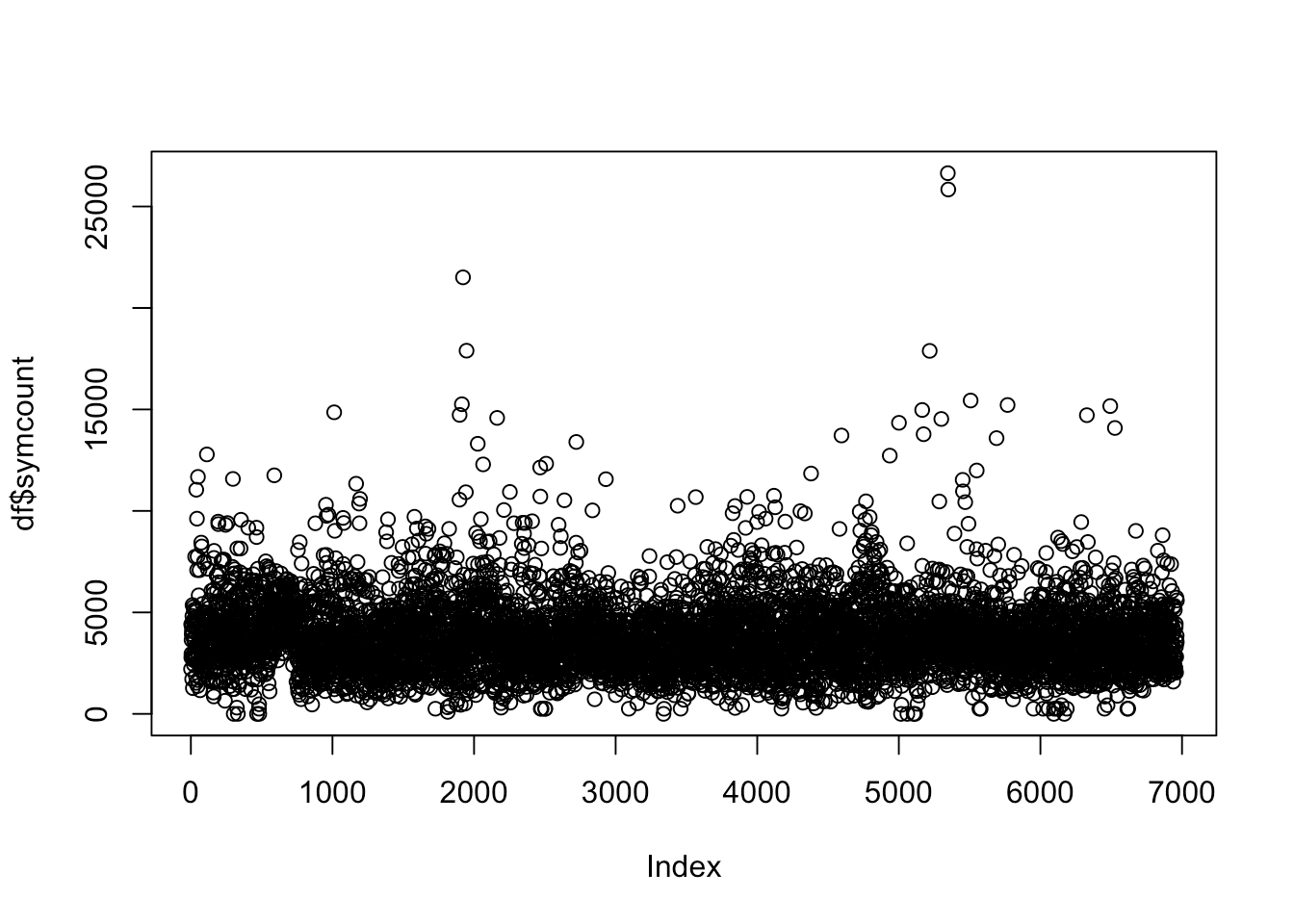
Let’s look at the symcount for the top 4 companies in our data set. We'll start by creating a new data frame that contains only the top four companies (which we can get from our summary() results), and then pass that data frame to plot() with our x and y values (company and symcount, respectively) as two separate arguments.
top4 <- names(summary(df$company)[1:4]) #get names of top 4 companies
justtop4 <- df[df$company
justtop4$company <- factor(justtop4$company) # make sure there are only 4 levels in our new factor

plot(justtop4$company, justtop4$symcount)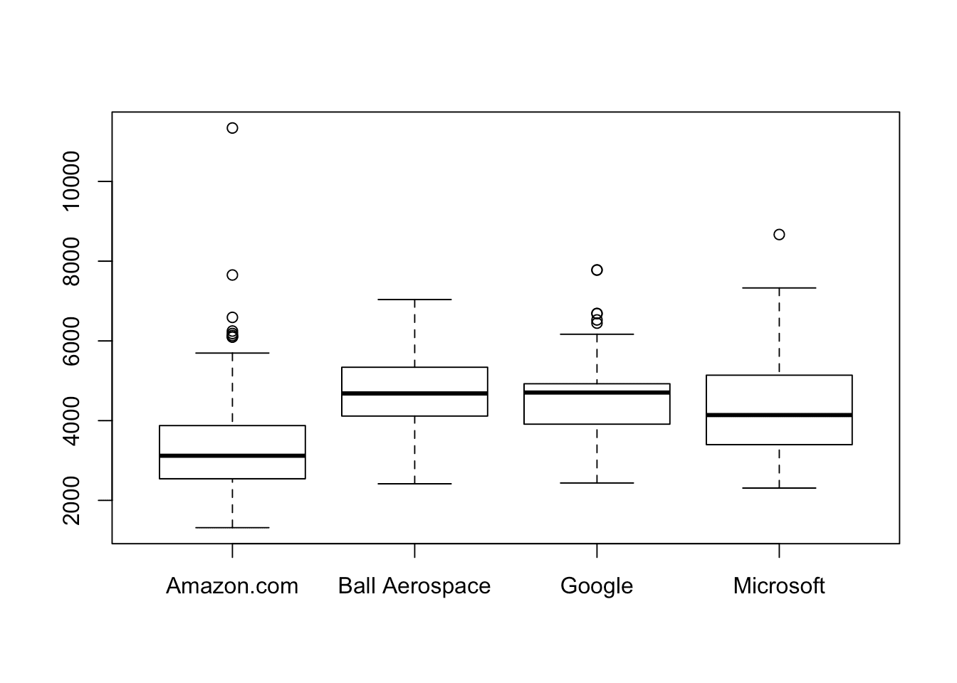
We can also run an Analysis of Variance (ANOVA) to see whether there is a statistically significant difference between the symcount of the 4 companies. R has a built-in function for this, too!
We'll create the ANOVA model using the aov() function, and then we call summary() and plot() on that model. These are the same functions we’ve been using, and even if we haven’t mastered what an ANOVA is yet, we can see that the output is different than what we saw before.
summary() and plot() (as mentioned before) are examples of generic functions in R. Generic functions create different outputs for different classes of objects. When we plotted symcount alone (a numeric vector), plot() gave us a scatterplot. When we plotted reviews (a numeric vector) and company (a categorical vector), plot() created a boxplot. When we plot an aov object (created by the aov() function), it gives us a series of plots that help us assess our model.
ANOVA <- aov(symcount ~ company, data = justtop4)
summary(ANOVA)
## Df Sum Sq Mean Sq F value Pr(>F)
## company 3 322841803 107613934 95.02 <2e-16 ***
## Residuals 812 919674198 1132604
## ---
## Signif. codes: 0 '***' 0.001 '**' 0.01 '*' 0.05 '.' 0.1 ' ' 1par(mfrow = c(2,2)) #lets us see all 4 plots at once!
plot(ANOVA)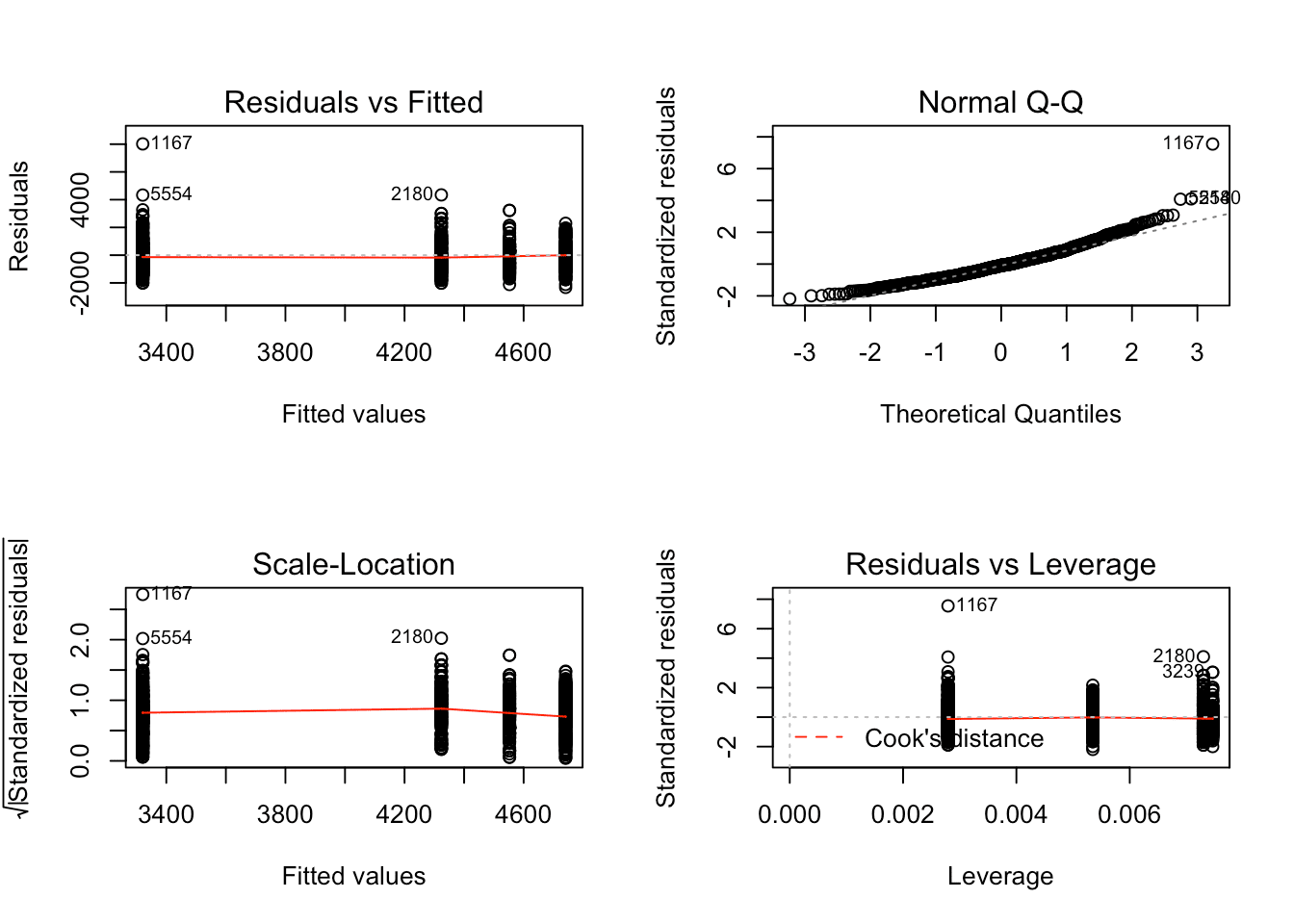
summary() on a dataframe, it provided a table of summary statistics for each column in the dataframe. When called on an aov object, summary() provides an ANOVA table.
Generic functions like these are incredibly helpful because they allow us to use the same function with the same syntax on a variety different objects in R and have the output be tailored to exactly what we need based on the object class. Instead of having to memorize a dozen slightly different functions for different classes, we can fall back on these trusty generic functions, which work for all of our classes.
We can better understand generic functions by imagining a function called feed(). Since generic functions offer different output based on the class that's input as an argument, we might expect feed(cat) to produce cat food, and feed(dog) to produce dog food. If we were to input feed(Chelsea), I hope this imaginary function would make me Waffle Fries.
Writing R Functions
While R has some very cool and complex generic functions, there isn't always going to be a built-in function for generating the output we want. Writing custom functions is an important part of programming, including programming in R.
As with vectorization, writing our own functions can streamline and speed up our code! As a general rule, if we find ourselves doing the same (or a similar) thing over and over, it might be time to write a function.
Syntax
To create a new R function we need to think about 4 major things:
- the name of the function
- the arguments (inputs) the function will take
- the code the function will run
- the output the function will return for the user
To see these four things in action, let’s write our own function to see whether the job descriptions in our data set mention a PhD.
We’ll start by giving it a clear name: phdFinder(). We'll create a variable called phdFinder to store our function. To create a function, we use function(){}.
phdFinder <- function(){

}
Above, the parentheses are empty, but that's where we will list the names for any arguments (inputs) that our function will need to run. Arguments are used to pass R objects/variables from outside the function into the function.
When choosing our arguments, it helps to ask: “which variables might be different each time this function is run?”. If a variable is likely to change, it should probably be specified as an argument rather than hard-coded inside the code the function will run.
In our function, the only thing that will be different is job description, so we’ll add a variable called description as an argument.
phdFinder <- function(description){
}
Next, we need to consider the code that the function will run. This is what we want the function to do to the argument or arguments we've passed it. For now, we’ll assume that we’re only looking for the string “PhD”, and that any other capitalization like “PHD” won’t count, so we'll want the code inside our function to look at each description it gets passed to see if it finds that string.
grepl() is a built-in R function looks for a smaller string of characters (like "PhD") inside a larger one (like our description). It will return TRUE if “PhD” is in the description, and FALSE if it was not. Let's add this to our function code, and assign the result of its assessment to a variable called mentioned.
phdFinder <- function(description){
  mentioned <- grepl("PhD",description)
}
The last thing we need to think about is what we want our function to return. Here, we want it to return mentioned, which will tell the user whether each description includes "PhD" (in which case mentioned will be TRUE) or not (in which case mentioned will be FALSE.
By default, R will return the value of the last statement we ran. phdFinder() only has one statement, so by default our function will return mentioned, with no extra work necessary! But if we wanted to explicitly tell R what to return, we could use the return() function.
If we do use return(), though, we need to be careful. The return() function tells R that the function is done running. So once that code runs, the function will stop.
To demonstrate this, let's add a return() line and then add a couple of print statements after it.
phdFinder <- function(description){
  print("checking...")
  mentioned <-  grepl("PhD",description)
  return(mentioned)
  print("YOU SEARCHED FOR A PHD!")
}
Note that running this code produces no output — the print statement is never run, because R stops executing the function at return(mentioned).
Using R Functions
Now that we’ve written our custom function, let’s try it out! We didn’t just write it for kicks and giggles. Let's take a look at the first job description in our original data set (stored as the data frame df) and check to see whether or not that job requires a PhD.
phdFinder(df[1,"description"])## [1] "checking..."
## [1] FALSEIt looks like there's no mention of a PhD in that job description. That's great news if we want a job that doesn’t require one.
Notice again that only the first print statement ran, not the second. As mentioned before, once the return() function is called, none of the following code will run.
We can also use our phdFinder() function on the entire column of descriptions at once. Yup, it’s automatically vectorized!
Let's create a new column in df called phd and store the results of calling phdFinder() on df$description there.
df$phd <- phdFinder(df$description)
head(df$phd)

print(sum(df$phd)/length(df$phd))
## [1] "checking..."
## [1] FALSE FALSE FALSE FALSE TRUE FALSE
## [1] 0.241527924
In the real world, we'd probably want to write some additional code to account for variant spellings like "PHD", "Ph.D", "phd", etc., before we draw any serious conclusions from this data.
We skipped that step in the code we've written here to make what's going on with our functions a bit easier to understand, but if you want to get more practice writing functions, rewriting our function with more complex code that accounts for these variants would be a great next step! Hint: you might want to start by looking into functions called tolower() and gsub().
Writing Good R Functions
Now that we know a little bit about how to write an R function, it’s time we had the talk. The talk about how to write good R functions.
First of all, we should write R functions as if someone else is going to be using them, because often they will be! But even if no one else is going to be using our code, we might want to re-use it later, so writing readable code is always a good idea.
Variable Names and Comments
Part of writing readable code means choosing argument and variable names that make sense. Don’t just use random letters (something I might be guilty of doing sometimes), use something meaningful.
For example, above we chose the variable name mentioned because this variable tells us whether “PhD” was mentioned. We could have called it x or weljhf, but by calling it mentioned we help ourselves and others better understand what’s being stored in that variable.
Similarly, giving our function a descriptive name like phdFinder() can help communicate what the function does. If we called this function something more cryptic, like function_47() or pf(), someone else reading our code would have a hard time figuring out what it does at a glance.
Scoping
This includes objects we’ve loaded as part of loading a library(). When we use a variable x, R will look around the room we’re in to find the value of x (we can check what’s in our environment using ls()).
When we write and run a function, R creates a new, temporary environment for the function. This is sort of like having a box in our room. The “box” holds all the objects we’ve created, changed, and used inside the function. But once the function is finished running, that box disappears.
Let’s look at a few examples to get a better idea of how this works. We'll run a few different snippets of code. In each case, we'll create an object (either a vector or a data frame) and pass it to our function, square, which returns the square of the number or numbers we passed it.
Note in the code below how the value of the variable x changes depending on whether it's outside the function (a global variable) or whether it's inside the function. The value of x can be reassigned within the function, but since the function environment is temporary and stops existing after the function is run, the global value of x doesn't change:
x <- 10
print(paste("Outside the function, x is...", x))

square <- function(y){
  x <- y**2
  print(paste("Inside the function, x is...", x))
}

square(x)
print(paste("Outside the function, x is...", x))
## [1] "Outside the function, x is... 10"
## [1] "Inside the function, x is... 100"
## [1] "Outside the function, x is... 10"x <- c(1,2,3)
print(paste("Outside the function, x is...", x[1],x[2],x[3]))
square <- function(y){
x <- y**2
print(paste("Inside the function, x is...", x[1],x[2],x[3]))
}
square(x)
print(paste("Outside the function, x is...", x[1],x[2],x[3]))## [1] "Outside the function, x is... 1 2 3"
## [1] "Inside the function, x is... 1 4 9"
## [1] "Outside the function, x is... 1 2 3"x <- data.frame(a = c(1,2,3))
print("Outside the function, x is...")
print(x)
square <- function(y){
x$square <- x$a**2
print("Inside the function, x is...")
print(x)
}
square(x)
print("Outside the function, x is...")
print(x)## [1] "Outside the function, x is..."
## a
## 1 1
## 2 2
## 3 3
## [1] "Inside the function, x is..."
## a square
## 1 1 1
## 2 2 4
## 3 3 9
## [1] "Outside the function, x is..."
## a
## 1 1
## 2 2
## 3 3To write good R functions, we need to think about where the objects we’re working with are. If there’s something outside the function environment that we want to use inside it, we can bring it in by passing it as an argument to our function.
If we don’t, R will look outside the “box” and search for the variable in the global environment (the “room”). But in order to make our function as generalizable as possible, and to avoid any issues with naming two variables the same thing, it’s a good idea to explicitly give our R function the objects it needs to run by passing them as arguments.
Getting Things Inside A Function
Let's take a look at what happens when we call a global variable inside a function without explicitly passing it as an argument. To do this, we'll create a new function called wordFinder(), similar to our phdFinder().
We'll write this function to make it look for the variable my_test_word in each job description. But my_test_word doesn’t exist inside the function environment, because it isn’t passed in as an argument, nor created inside the function. So what will happen?
Once R searches this local environment and comes up empty, it will search the global environment for my_test_word. Since my_test_word exists in the global environment, R will use that inside the function.
my_test_word <- "python" #R uses "python" for my_test_word because it can't find my_test_word in the local function environment

wordFinder <- function(description){
  print(paste("checking for...", my_test_word))
  mentioned <-  grepl(my_test_word,description)
  return(mentioned)

}

wordFinder(df[1,"description"])
## [1] "checking for... python"## [1] FALSE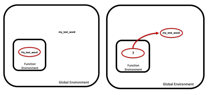
my_test_word twice, both inside and outside the function? Let's give it a shot!
Outside the function, in the global environment, we'll give my_test_word the value 'python'. Inside the function, we'll assign it the value 'data'.
Since we already know that R searches the function environment before the global environment, we might predict that R will use 'data' as the value of my_test_word, since that's the value that's assigned inside the function. Indeed, that's what happens:
my_test_word <- "python"

wordFinder <- function(description){
  my_test_word <- "data" #R uses "data" for my_test_word because it searches the local environment first
  print(paste("checking for...", my_test_word))
  mentioned <-  grepl(my_test_word,description)
  return(mentioned)

}

wordFinder(df[1,"description"])
## [1] "checking for... data"
## [1] TRUEWhen we run this code block, we can see that R uses 'data' (the value of my_test_word inside the function) rather than 'python'. When my_test_word was referenced in grepl(), R first searched the local function environment and found my_test_word. So it didn’t need to search the global environment at all.
This is important to keep in mind when writing functions: R will only search the global environment for a variable if it doesn't find that variable in the function environment (either as an argument or as a variable defined within the function itself).
Getting Things Out of a Function
It’s nice that R tidies up for us by removing the local function environment after a function has run, but what if we want to keep something a value generated inside a function after the function has run?
We can keep things created or changed inside the function by returning them. When we return a variable from a function, it allows us to store it in the global environment (if we so choose).
In wordFinder(), we return mentioned. Since R removed the local function environment, mentioned doesn’t exist anymore. When we try to print it out, we get an error.
my_test_word <- "python"

wordFinder <- function(description){
  my_test_word <- "data" #R uses "data" for my_test_word because it searches the local environment first
  print(paste("checking for...", my_test_word))
  mentioned <-  grepl(my_test_word,description)
  return(mentioned)

}

wordFinder(df[1,"description"])
print(mentioned)
## Error in print(mentioned): object 'mentioned' not found## [1] "checking for... data"
## [1] TRUEHowever, since wordFinder() returns the value of mentioned, we can store it in our global environment by assigning the output of our function to a variable. Now we can use that value outside the function.
my_test_word <- "python"

wordFinder <- function(description){
  my_test_word <- "data" #R uses "data" for my_test_word because it searches the local environment first
  print(paste("checking for...", my_test_word))
  mentioned <-  grepl(my_test_word,description)
  return(mentioned)

}

mentioned2 <- wordFinder(df[1,"description"])
print(mentioned2)
## [1] "checking for... data"
## [1] TRUENow we've got the value from inside the function preserved outside of it.
In Review:
Functions in R have a lot of uses, so let’s debrief with a few bullet points:
- R functions are pieces of code that take inputs, called arguments, and turn them into outputs.
- Arguments go inside a function's parentheses both when we define a function and anytime we call a function.
- Outputs are the objects that are returned by the function.
- By default R will return the value of the last statement in the function. Everything else that may have been changed or created in the function will disappear once the function is done running unless we intentionally take steps to preserve it.
- R Functions are made to be used over and over. This saves us time, space, and makes our code look better.
- R Functions are often vectorized, which means that we can run the function for each item in a vector, like a column of data in a data frame, all in one go! This often saves a lot of time.
- Generic R Functions are functions that run differently based on the class of the object passed to it as an argument.
- Writing good R functions means thinking of others (and our future selves) and to make our functions easy to understand.
Now that you've got a solid understanding of the fundamentals of R functions, add to your skillset with Dataquest's free, interactive R courses. Our Intermediate course will take you even deeper into the world of functions, all while letting you write code from right in your browser.