Working with Large Datasets using Pandas and JSON in Python
Working with large JSON datasets can feel overwhelming, especially when they’re too large to fit into memory. Fortunately, combining Python with tools like Pandas can make exploring and analyzing even massive datasets manageable. In this post, we’ll focus on how to use Python and JSON to tackle a real-world problem: mapping out police activity in Montgomery County, Maryland. We’ll start by examining the JSON data and then dive into exploration and analysis using Pandas.
When data is stored in SQL databases, it typically follows a rigid, tabular structure. Here’s an example of a dataset stored in a SQLite database, where each row represents a country, and each column captures details like population, area, or growth rates:
| id | code | name | area | area_land | area_water | population | population_growth | birth_rate | death_rate | migration_rate | created_at | updated_at |
|---|---|---|---|---|---|---|---|---|---|---|---|---|
| 1 | af | Afghanistan | 652230 | 652230 | 0 | 32564342 | 2.32 | 38.57 | 13.89 | 1.51 | 2015-11-01 13:19:49.461734 | 2015-11-01 13:19:49.461734 |
| 2 | al | Albania | 28748 | 27398 | 1350 | 3029278 | 0.3 | 12.92 | 6.58 | 3.3 | 2015-11-01 13:19:54.431082 | 2015-11-01 13:19:54.431082 |
| 3 | ag | Algeria | 2381741 | 2381741 | 0 | 39542166 | 1.84 | 23.67 | 4.31 | 0.92 | 2015-11-01 13:19:59.961286 | 2015-11-01 13:19:59.961286 |
As you can see, the data is structured into rows and columns, making it easy to query specific facts, like a country’s population or growth rate.
As the amount of data we collect grows, we often encounter unstructured data—data that doesn’t follow a consistent or predefined format. A good example is a list of events captured from website visitors. Unlike the tabular format of SQL databases, unstructured data can vary in structure and often includes nested fields. This makes it challenging to store and query in a traditional database.
Here’s an example of unstructured data in the form of events sent to a server, stored in JavaScript Object Notation (JSON):
{
  "event_type": "started-lesson",
  "keen": {
    "created_at": "2015-06-12T23:09:03.966Z",
    "id": "557b668fd2eaaa2e7c5e916b",
    "timestamp": "2015-06-12T23:09:07.971Z"
  },
  "sequence": 1
},
{
  "event_type": "started-screen",
  "keen": {
    "created_at": "2015-06-12T23:09:03.979Z",
    "id": "557b668f90e4bd26c10b6ed6",
    "timestamp": "2015-06-12T23:09:07.987Z"
  },
  "lesson": 1,
  "sequence": 4,
  "type": "code"
},
{
  "event_type": "started-screen",
  "keen": {
    "created_at": "2015-06-12T23:09:22.517Z",
    "id": "557b66a246f9a7239038b1e0",
    "timestamp": "2015-06-12T23:09:24.246Z"
  },
  "lesson": 1,
  "sequence": 3,
  "type": "code"
}
In this example, each JSON object represents a separate event. Some fields, like keen, are nested within other fields. This flexible structure makes JSON a popular format for storing unstructured data, as it can easily represent complex relationships. Despite its name, JSON isn’t limited to JavaScript—Python’s json module makes it simple to read, write, and process JSON data.
Python makes working with JSON data straightforward, thanks to its built-in json library. With it, you can easily convert JSON strings into Python lists or dictionaries, and vice versa. This is especially useful since JSON data closely resembles Python dictionaries, with key-value pairs that are simple to navigate and manipulate.
In this post, we’ll start by exploring a JSON file using the command line. Then, we’ll import it into Python and use Pandas to analyze the data efficiently.
The Dataset
We’ll be looking at a dataset that contains information on traffic violations in Montgomery County, Maryland. You can download the data here. The data contains information about where the violation happened, the type of car, demographics on the person receiving the violation, and some other interesting information. There are quite a few questions we could answer using this dataset, including:
- What types of cars are most likely to be pulled over for speeding?
- What times of day are police most active?
- How common are “speed traps”? Or are tickets spread pretty evenly in terms of geography?
- What are the most common things people are pulled over for?
Unfortunately, we don’t know the structure of the JSON file upfront, so we’ll need to do some exploration to figure it out. We’ll use Jupyter Notebook for this exploration.
Exploring the JSON Data
Even though the JSON file is only 600MB, we’ll treat it like it’s much larger to simulate how analyzing a JSON file that doesn’t fit into memory might work. The first thing we’ll do is take a look at the first few lines of the md_traffic.json file. A JSON file is just an ordinary text file, so we can use standard command line tools to interact with it:
head md_traffic.json
{
  "meta": {
    "view": {
      "id": "4mse-ku6q",
      "name": "Traffic Violations",
      "averageRating": 0,
      "category": "Public Safety",
      "createdAt": 1403103517,
      "description": "This dataset contains traffic violation information from all electronic traffic violations issued in the County. Any information that can be used to uniquely identify the vehicle, the vehicle owner, or the officer issuing the violation will not be published.",
      "Update Frequency": "Daily",
      "displayType": "table"
    }
  }
}
From this snippet, we can see that the JSON data is structured as a dictionary. The top-level key is meta, which contains another dictionary as its value. Keys and values are indented by two spaces, which makes the JSON well-formatted and easy to read.
Exploring the Top-Level Keys
To identify all the top-level keys in the md_traffic.json file, we can use the grep command. Specifically, we’ll look for lines that start with two spaces followed by a quotation mark, which indicates the presence of a key:
grep -E '^ {2}"' md_traffic.jsonThe command outputs something like this:
"meta": {
  "view": {
    "id": "4mse-ku6q",
    "name": "Traffic Violations",
    "category": "Public Safety"
  }
},
"data": [
  [
    1889194,
    "92AD0076-5308-45D0-BDE3-6A3A55AD9A04",
    1455876689,
    "2016-02-18T00:00:00",
    "DRIVER USING HANDS TO USE HANDHELD TELEPHONE WHILE MOTOR VEHICLE IS IN MOTION",
    "355/TUCKERMAN LN",
    "MD",
    "Citation",
    "21-1124.2(d2)",
    "Transportation Article"
  ]
]
This output shows that the top-level keys in the md_traffic.json file are meta and data. The meta key contains metadata about the dataset, while data holds the actual traffic violations records.
The data key appears to be associated with a list of lists, where each inner list represents a single record. From the output above, we can see one such record, which includes fields like a violation description, location, and citation details. This structure is similar to the kind of tabular data we often work with in CSV files or SQL tables, making it easier to process using tools like Pandas.
Here’s a truncated view of how the data might look:
[
  [1889194, "92AD0076-5308-45D0-BDE3-6A3A55AD9A04", 1889194, 1455876689, "498050"],
  [1889194, "92AD0076-5308-45D0-BDE3-6A3A55AD9A04", 1889194, 1455876689, "498050"],
  ...
]
This structure resembles the rows and columns we’re used to working with in tables. Each inner list represents a row of data, but we’re missing the headers that tell us what each column represents. Fortunately, this information might be available under the meta key in the JSON file.
Exploring the meta Key
The meta key usually contains information about the data itself. Let’s take a closer look at what’s stored under meta. From the earlier head command, we know that meta contains a nested structure, including a key view with attributes like id, name, and averageRating. To see the full structure of the JSON file, we can use grep to extract all lines with 2 to 6 leading spaces, which often correspond to nested keys:
grep -E '^ {2,6}"' md_traffic.jsonThe output shows the following:
"meta": {
  "view": {
    "id": "4mse-ku6q",
    "name": "Traffic Violations",
    "averageRating": 0,
    "category": "Public Safety",
    "createdAt": 1403103517,
    "description": "This dataset contains traffic violation information. Any information that uniquely identifies vehicles, owners, or officers will not be published.",
    "displayType": "table",
    "columns": [
      {
        "name": "Violation Description",
        "dataType": "text"
      },
      {
        "name": "Location",
        "dataType": "text"
      },
      {
        "name": "Date Issued",
        "dataType": "date"
      }
    ]
  }
}
This output reveals the full key structure associated with meta. Notably, the columns key looks promising—it likely contains metadata about the columns in the list of lists within the data key. This will be important for understanding the structure of our dataset as we proceed with analysis.
Extracting Information on the Columns
Now that we’ve identified which key contains information about the columns, we need to extract that information. Because the JSON file is too large to fit into memory, we can’t simply load it using the built-in json library. Instead, we’ll use a memory-efficient approach to iteratively read the data.
The ijson package is perfect for this task. Unlike the standard json library, ijson parses the JSON file incrementally, reading it one piece at a time. While this approach is slower, it allows us to handle large files without running out of memory. Here’s how to use ijson to extract column metadata:
import ijson

filename = "md_traffic.json"
with open(filename, 'r') as f:
    # Extract items from the specified path
    objects = ijson.items(f, 'meta.view.columns.item')
    columns = list(objects)
In this code:
- We open the
md_traffic.jsonfile in read mode. - The
itemsmethod fromijsonis used to extract data from the specified path,meta.view.columns.item. - The path
meta.view.columns.itemspecifies that we’re extracting each individual item in thecolumnslist, located undermeta.view. - The extracted items are converted to a list using
list(objects), allowing us to work with them directly in Python.
This method ensures that we can efficiently extract the column information from large JSON files without loading the entire file into memory.
Extracting Column Names
The items function in ijson returns a generator, so we use the list method to convert it into a Python list. To inspect the metadata for a single column, we can print the first item in the list:
print(columns[0])The output might look something like this:
{
  "renderTypeName": "meta_data",
  "name": "sid",
  "fieldName": ":sid",
  "position": 0,
  "id": -1,
  "format": {},
  "dataTypeName": "meta_data"
}
Each item in columns is a dictionary containing metadata about a specific column. To extract the column names, the fieldName key appears to hold the relevant information. We can create a list of column names by iterating through columns and extracting this key:
column_names = [col["fieldName"] for col in columns]
column_names
The resulting list will look like this:
[
  ":sid", ":id", ":position", ":created_at", ":created_meta", ":updated_at", ":updated_meta", ":meta",
  "date_of_stop", "time_of_stop", "agency", "subagency", "description", "location", "latitude", "longitude",
  "accident", "belts", "personal_injury", "property_damage", "fatal", "commercial_license", "hazmat",
  "commercial_vehicle", "alcohol", "work_zone", "state", "vehicle_type", "year", "make", "model", "color",
  "violation_type", "charge", "article", "contributed_to_accident", "race", "gender", "driver_city",
  "driver_state", "dl_state", "arrest_type", "geolocation"
]
With the column names extracted, we’re now ready to move on to extracting the actual data from the JSON file.
Extracting the Data
The data we need is stored in a list of lists under the data key. To work with it efficiently, we can extract only the columns we care about using the column names we retrieved earlier. This selective extraction will save memory and space. For very large datasets, you could process the data in batches—for example, reading 10 million rows at a time, processing them, and then moving to the next batch.
In this example, we’ll define a list of relevant columns and use ijson to iteratively extract the data:
good_columns = [
    "date_of_stop", "time_of_stop", "agency", "subagency", "description",
    "location", "latitude", "longitude", "vehicle_type", "year",
    "make", "model", "color", "violation_type", "race", "gender",
    "driver_state", "driver_city", "dl_state", "arrest_type"
]

data = []
with open(filename, 'r') as f:
    objects = ijson.items(f, 'data.item')
    for row in objects:
        # Select only the relevant columns
        selected_row = [
            row[column_names.index(item)]
            for item in good_columns
        ]
        data.append(selected_row)
Here’s what this code does:
good_columns: Defines the list of columns we’re interested in.ijson.items: Iteratively reads the rows from thedatakey in the JSON file.selected_row: Extracts only the values corresponding to thegood_columnsfrom each row.data.append: Adds the filtered row to thedatalist.
Once the data is extracted, we can inspect the first row to confirm that it matches our expectations:
print(data[0])The output will look like this:
[
  "2016-02-18T00:00:00", "09:05:00", "MCP", "2nd district, Bethesda",
  "DRIVER USING HANDS TO USE HANDHELD TELEPHONE WHILE MOTOR VEHICLE IS IN MOTION",
  "355/TUCKERMAN LN", "-77.105925", "39.03223", "02 - Automobile", "2010",
  "JEEP", "CRISWELL", "BLUE", "Citation", "WHITE", "F", "MD", "GERMANTOWN",
  "MD", "A - Marked Patrol"
]
Great! We now have the filtered data stored in memory and ready for further processing.
Reading the Data into Pandas
Now that we have the data as a list of lists and the column headers as a list, we can load it into a Pandas DataFrame for analysis. If you’re unfamiliar with Pandas, it’s a powerful data analysis library that provides an efficient, tabular data structure called a DataFrame. Pandas allows us to easily convert a list of lists into a DataFrame and specify column names separately:
import pandas as pd

# Create a DataFrame from the data
stops = pd.DataFrame(data, columns=good_columns)
With the data in a DataFrame, we can quickly perform analysis. For example, here’s how we can calculate the number of stops for each car color:
stops["color"].value_counts()The output will look like this:
BLACK           161319
SILVER          150650
WHITE           122887
GRAY             86322
RED              66282
BLUE             61867
GREEN            35802
GOLD             27808
TAN              18869
BLUE, DARK       17397
MAROON           15134
BLUE, LIGHT      11600
BEIGE            10522
GREEN, DK        10354
N/A               9594
GREEN, LGT        5214
BROWN             4041
YELLOW            3215
ORANGE            2967
BRONZE            1977
PURPLE            1725
MULTICOLOR         723
CREAM              608
COPPER             269
PINK               137
CHROME              21
CAMOUFLAGE          17
dtype: int64
Interestingly, camouflage doesn't seem to be a very popular car color!
Analyzing Police Units Creating Citations
Next, let’s look at the types of police units responsible for creating citations. We can use Pandas to count the occurrences of each type in the arrest_type column:
stops["arrest_type"].value_counts()The output will look like this:
A - Marked Patrol                  671165
Q - Marked Laser                    87929
B - Unmarked Patrol                 25478
S - License Plate Recognition       11452
O - Foot Patrol                      9604
L - Motorcycle                       8559
E - Marked Stationary Radar          4854
R - Unmarked Laser                   4331
G - Marked Moving Radar (Stationary) 2164
M - Marked (Off-Duty)                1301
I - Marked Moving Radar (Moving)      842
F - Unmarked Stationary Radar         420
C - Marked VASCAR                     323
D - Unmarked VASCAR                   210
P - Mounted Patrol                    171
N - Unmarked (Off-Duty)               116
H - Unmarked Moving Radar (Stationary) 72
K - Aircraft Assist                    41
J - Unmarked Moving Radar (Moving)     35
dtype: int64
Despite the rise of technologies like red light cameras and speed lasers, patrol cars remain the dominant source of citations by a significant margin. This highlights their continued importance in enforcing traffic laws.
Converting Columns
To perform time- and location-based analysis, we need to convert the longitude, latitude, and date columns from strings to appropriate numerical types. Let’s start with longitude and latitude. We can use the following code to convert these columns to floats:
import numpy as np

# Define a function to safely parse strings to floats
def parse_float(x):
    try:
        return float(x)
    except ValueError:
        return 0.0

# Apply the function to the longitude and latitude columns
stops["longitude"] = stops["longitude"].apply(parse_float)
stops["latitude"] = stops["latitude"].apply(parse_float)
This ensures that any invalid values in the longitude or latitude columns are replaced with 0.0, making the data safe for analysis.
Interestingly, the time and date of each stop are stored in two separate columns: time_of_stop and date_of_stop. We’ll need to address this separation to analyze datetime information effectively, which we’ll handle in the next step.
Parsing and Analyzing Datetimes
To analyze time- and date-based trends, we need to combine the date_of_stop and time_of_stop columns into a single datetime column. Here’s how we can achieve this using the datetime module:
from datetime import datetime

# Function to combine date and time into a single datetime object
def parse_full_date(row):
    # Parse the date string
    date = datetime.strptime(row["date_of_stop"], "%Y%m%dT%H%M%S")
    # Split the time string and update the datetime object
    time = row["time_of_stop"].split(":")
    date = date.replace(
        hour=int(time[0]),
        minute=int(time[1]),
        second=int(time[2])
    )
    return date

# Apply the function to create a new datetime column
stops["date"] = stops.apply(parse_full_date, axis=1)
Now that we have a single datetime column, we can visualize traffic stops by day of the week. Using Matplotlib, we can plot a histogram to see which days have the most stops:
import matplotlib.pyplot as plt
# Enable inline plotting for Jupyter Notebook
%matplotlib inline
# Plot histogram of traffic stops by weekday
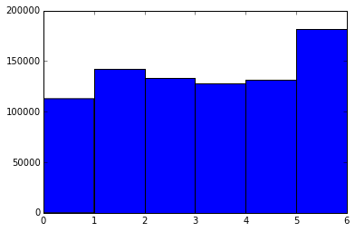
plt.hist(stops["date"].dt.weekday, bins=6)
plt.xlabel("Day of the Week")
plt.ylabel("Number of Stops")
plt.title("Traffic Stops by Day of the Week")
plt.show()
The histogram output will look something like this:
(array([112816., 142048., 133363., 127629., 131735., 181476.]),
 array([0., 1., 2., 3., 4., 5., 6.]),
 <a list of 6 Patch objects>)
This plot shows how traffic stops vary by day of the week, with certain days experiencing significantly higher enforcement activity.
Analyzing Stop Times
In the previous plot, Monday is represented as 0 and Sunday as 6. It appears that Sunday has the highest number of stops, while Monday has the fewest. This pattern might reflect actual enforcement trends, but it could also point to a data quality issue—invalid or missing dates may default to Sunday. Investigating the date_of_stop column further would be necessary to confirm this, but that’s beyond the scope of this post.
We can also analyze the most common times of day for traffic stops. Here’s a histogram of traffic stops by hour:
plt.hist(stops["date"].dt.hour, bins=24)
plt.xlabel("Hour of the Day")
plt.ylabel("Number of Stops")
plt.title("Traffic Stops by Hour of the Day")
plt.show()
The histogram output might look like this:
(array([ 44125., 35866., 27274., 18048., 11271.,  7796., 11959., 29853.,
         46306., 42799., 43775., 37101., 34424., 34493., 36006., 29634.,
         39024., 40988., 32511., 28715., 31983., 43957., 60734., 60425.]),
 array([ 0.,  1.,  2.,  3.,  4.,  5.,  6.,  7.,  8.,  9., 10., 11., 12.,
         13., 14., 15., 16., 17., 18., 19., 20., 21., 22., 23., 24.]),
 <a list of 24 Patch objects>)
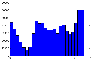
The plot shows that the highest number of stops occurs around midnight, with the fewest happening around 5 a.m. This makes sense—late-night hours often coincide with increased enforcement as people drive home from bars or dinners. However, as with the day-of-week analysis, this trend could also reflect data quality issues. A closer examination of the time_of_stop column would help determine whether the pattern is genuine.
Subsetting the Stops
Now that we’ve converted the location and date columns, we can start mapping the traffic stops. Since mapping is resource-intensive, we’ll first filter down the dataset to include only relevant rows. For example, we can subset the data to include stops from the past year:
from datetime import datetime

# Filter stops from the past year
last_year = stops[stops["date"] > datetime(year=2015, month=2, day=18)]
In this code, we select all rows where the date column is greater than February 18, 2015. To further narrow down the data, we can filter for stops that occurred during the morning rush hours (weekdays between 6 a.m. and 9 a.m.):
# Filter for weekday morning rush hours
morning_rush = last_year[
    (last_year["date"].dt.weekday < 5) &  # Weekdays only
    (last_year["date"].dt.hour > 5) &    # After 5 a.m.
    (last_year["date"].dt.hour < 10)     # Before 10 a.m.
]

# Display the shapes of the subsets
print("Morning rush shape:", morning_rush.shape)
print("Last year shape:", last_year.shape)
The output of the shape method shows the dimensions of the filtered data:
Morning rush shape: (29824, 21)
Last year shape: (234582, 21)
By subsetting the data this way, we’ve reduced the size of the dataset significantly, making it easier to analyze and map traffic stops efficiently.
Mapping Traffic Stops
We can now visualize the locations of traffic stops using the excellent folium package. Folium makes it easy to create interactive maps in Python by leveraging Leaflet. To preserve performance, we’ll only map the first 1000 rows of the morning_rush dataset.
import folium
from folium.plugins import MarkerCluster

# Create a base map centered on Montgomery County, Maryland
stops_map = folium.Map(location=[39.0836, -77.1483], zoom_start=11)

# Add a marker cluster to the map
marker_cluster = MarkerCluster().add_to(stops_map)

# Add markers for the first 1000 rows of the morning_rush dataset
for _, row in morning_rush.iloc[:1000].iterrows():
    folium.Marker(
        location=[row["latitude"], row["longitude"]],
        popup=row["description"]
    ).add_to(marker_cluster)

# Save the map to an HTML file
stops_map.save('stops.html')

# Display the map in the notebook (if supported)
stops_map
In this code:
folium.Map: Creates a base map centered on Montgomery County, Maryland, with a zoom level of11.MarkerCluster: Groups markers into clusters to improve performance and map readability.folium.Marker: Adds individual markers for each traffic stop, using thelatitudeandlongitudecolumns for location and thedescriptioncolumn for popup information.stops_map.save: Saves the map to an HTML file so you can view it in your browser.
After running this code, you’ll get an interactive map where you can explore the locations and descriptions of traffic stops during the morning rush. The map is saved as stops.html and can be opened in any web browser.
Creating a Heatmap
To visualize traffic stop density, we can create a heatmap using the HeatMap plugin from Folium. Here’s the updated code:
from folium.plugins import HeatMap

# Create a base map centered on Montgomery County, Maryland
stops_heatmap = folium.Map(location=[39.0836, -77.1483], zoom_start=11)

# Add a heatmap layer using the first 1000 rows of morning_rush
heat_data = [[row["latitude"], row["longitude"]] for _, row in morning_rush.iloc[:1000].iterrows()]
HeatMap(heat_data).add_to(stops_heatmap)

# Save the heatmap to an HTML file
stops_heatmap.save("heatmap.html")

# Display the map in the notebook (if supported)
stops_heatmap
Here’s what the code does:
folium.Map: Initializes a base map centered on Montgomery County with a zoom level of11.HeatMap: Creates a heatmap layer using the latitude and longitude data from the first 1000 rows ofmorning_rush.save: Saves the resulting heatmap as an HTML file for viewing in a browser.
After running this code, the heatmap will be saved as heatmap.html. You can open the file in your browser to explore the density of traffic stops visually.
Next Steps
In this post, we focused on Python programming, and we learned how to use it to go from raw JSON data to fully functional maps using command line tools, ijson, Pandas, matplotlib, and folium. If you want to learn more about these tools, check out our Python Basics for Data Analysis, Data Analysis and Visualization with Python, and Command Line for Data Science courses.
If you want to further explore this dataset, here are some interesting questions to answer:
- Does the type of stop vary by location?
- How does income correlate with number of stops?
- How does population density correlate with number of stops?
- What types of stops are most common around midnight?