Published։ February 24, 2026

Project Tutorial: Predicting Employee Productivity with Decision Trees and Random Forests

In this project walkthrough, we'll build a machine learning model to predict whether a given workday in a garment factory will be productive or not. As a data scientist working with factory management, our goal is to analyze team-level productivity data and identify the key conditions that drive performance on the floor.

What makes this project especially rewarding is the end result: a visual decision tree you can actually show to non-technical stakeholders. Rather than presenting a black-box model, we'll be able to walk a factory manager through the exact questions the model asks to arrive at a prediction.

What You'll Learn

By the end of this tutorial, you'll know how to:

Clean and prepare real-world operational data for machine learning
Build and visualize a decision tree classifier using scikit-learn
Evaluate model performance using accuracy, precision, recall, F1 score, and cross-validation
Interpret a decision tree for a non-technical business audience
Use a random forest to validate your single-tree results

Before You Start

To make the most of this project walkthrough, follow these preparatory steps:

Review the Project
Access the project and familiarize yourself with the goals and structure: Predicting Employee Productivity Project.
Prepare Your Environment
- If you're using the Dataquest platform, everything is already set up for you.
- If you're working locally, ensure you have Python and Jupyter Notebook installed, along with pandas, matplotlib, and sklearn.
- Download the garments_worker_productivity.csv dataset from the project.
Prerequisites
- Comfortable with Python basics (loops, functions, data structures)
- Familiar with pandas DataFrames and basic data manipulation
- Some exposure to the machine learning workflow is helpful but not required

New to tree-based models? The Decision Tree and Random Forest Modeling in Python course covers the core concepts we'll apply here.

Setting Up Your Environment

Let's start by importing the libraries we'll need for exploration and visualization:

import pandas as pd
from matplotlib import pyplot as plt

We'll import scikit-learn modules later, closer to where we use them, which keeps things organized as the project grows.

Now let's load the dataset and take a first look:

df = pd.read_csv("garments_worker_productivity.csv")
df.head()

         date   quarter department        day  team  targeted_productivity    smv      wip  over_time  incentive  idle_time  idle_men  no_of_style_change  no_of_workers  actual_productivity
0  1/1/2015  Quarter1     sweing   Thursday     8                   0.80  26.16   1108.0       7080         98        0.0         0                   0           59.0             0.940725
1  1/1/2015  Quarter1   finishing  Thursday     1                   0.75   3.94      NaN        960          0        0.0         0                   0            8.0             0.886500
2  1/1/2015  Quarter1     sweing   Thursday    11                   0.80  11.41    968.0       3660         50        0.0         0                   0           30.5             0.800570
3  1/1/2015  Quarter1     sweing   Thursday    12                   0.80  11.41    968.0       3660         50        0.0         0                   0           30.5             0.800570
4  1/1/2015  Quarter1     sweing   Thursday     6                   0.80  25.90   1170.0       1920         50        0.0         0                   0           56.0             0.800382

Our dataset contains daily productivity records for teams across two departments of a garment factory. Here's what each column represents:

date: The date of the record (January to March of a single year)
quarter: A portion of the month (Quarter1 = Week 1, Quarter2 = Week 2, etc.)
department: The factory department (sewing or finishing)
day: Day of the week
team: A numeric identifier for each team (1–12)
targeted_productivity: The productivity target set for that day (0 to 1 scale)
smv: Standard Minute Value — the allocated time for a task, in minutes
wip: Work in Progress — tasks still pending
over_time: Overtime worked, in minutes
incentive: Financial incentive given to the team, in BDT
idle_time: Time lost due to production issues
idle_men: Number of workers who were idle
no_of_style_change: Number of product style changes that day
no_of_workers: Number of workers on the team
actual_productivity: The actual productivity achieved (0 to 1 scale, our basis for the target variable)

Learning Insight: Notice that quarter here does NOT mean a calendar quarter. It refers to a week within a month. This is the kind of domain-specific detail that's easy to miss but important to get right before modeling.

Exploratory Data Analysis (EDA)

Before we touch a single model, we need to understand what we're working with. Let's check the structure of the dataset:

df.info()

<class 'pandas.core.frame.DataFrame'>
RangeIndex: 1197 entries, 0 to 1196
Data columns (total 15 columns):
 #   Column                 Non-Null Count  Dtype
---  ------                 --------------  -----
 0   date                   1197 non-null   object
 1   quarter                1197 non-null   object
 2   department             1197 non-null   object
 3   day                    1197 non-null   object
 4   team                   1197 non-null   int64
 5   targeted_productivity  1197 non-null   float64
 6   smv                    1197 non-null   float64
 7   wip                    691 non-null    float64
 8   over_time              1197 non-null   int64
 9   incentive              1197 non-null   int64
 10  idle_time              1197 non-null   float64
 11  idle_men               1197 non-null   int64
 12  no_of_style_change     1197 non-null   int64
 13  no_of_workers          1197 non-null   float64
 14  actual_productivity    1197 non-null   float64
dtypes: float64(6), int64(5), object(4)
memory usage: 140.4+ KB

A few things stand out right away. The wip column has only 691 non-null values out of 1,197 rows, meaning roughly 42% of it is missing. We also have several object (string/categorical) columns that machine learning models can't use directly. We'll address both issues during cleaning.

Let's look at the categorical columns before diving into the numbers:

df["department"].value_counts()

department
sweing        691
finishing     257
finishing     249
Name: count, dtype: int64

Three rows for what should be two departments. Let's see why:

df["department"].unique()

array(['sweing', 'finishing ', 'finishing'], dtype=object)

Two data quality issues in one column: "sweing" is a typo for "sewing", and some "finishing" values have a hidden trailing space. Both need to be fixed.

df["quarter"].value_counts()

quarter
Quarter1    360
Quarter2    335
Quarter4    248
Quarter3    210
Quarter5     44
Name: count, dtype: int64

Quarter5 shows up with 44 entries. Since quarters represent weeks of a month, Quarter5 covers dates that fall on the 29th through 31st. With only 44 records, it's too sparse to stand on its own, so we'll merge it into Quarter4.

df["day"].value_counts()

day
Wednesday    208
Sunday       203
Tuesday      201
Thursday     199
Monday       199
Saturday     187
Name: count, dtype: int64

No Fridays in the dataset. The data spans January through March of a single year, so Friday may simply have been a non-working day. Either way, it won't significantly affect our model.

Now let's check the numeric distributions:

df.describe()

            team  targeted_productivity          smv          wip    over_time    incentive   idle_time    idle_men  no_of_style_change  no_of_workers  actual_productivity
count  1197.000000          1197.000000  1197.000000   691.000000  1197.000000  1197.000000  1197.000000  1197.000000         1197.000000    1197.000000          1197.000000
mean      6.426901             0.729632    15.062172   1190.465991  4567.460317    38.210526     0.730159     0.369256            0.150376      34.609858             0.735091
std       3.463963             0.097891    10.943219   1837.455001  3348.823563   160.182643    12.709757     3.268987            0.427848      22.197687             0.174488
min       1.000000             0.070000     2.900000      7.000000     0.000000     0.000000     0.000000     0.000000            0.000000       2.000000             0.233705
25%       3.000000             0.700000     3.940000    774.500000  1440.000000     0.000000     0.000000     0.000000            0.000000       9.000000             0.650307
50%       6.000000             0.750000    15.260000   1039.000000  3960.000000     0.000000     0.000000     0.000000            0.000000      34.000000             0.773333
75%       9.000000             0.800000    24.260000   1252.500000  6960.000000    50.000000     0.000000     0.000000            0.000000      57.000000             0.850253
max      12.000000             0.800000    54.560000  23122.000000 25920.000000  3600.000000   300.000000    45.000000            2.000000      89.000000             1.120437

Two things worth noting: the actual_productivity column has a maximum value above 1.0, even though the dataset documentation describes it as a 0-to-1 scale. We'll handle this by converting the column into a binary classification target rather than a regression target. Also, the mean incentive is about 38, but the median is 0, which tells us most days have no incentive at all — a heavily skewed distribution that the model will need to handle.

Let's look at the distributions visually:

df.hist(figsize=(10, 10))
plt.show()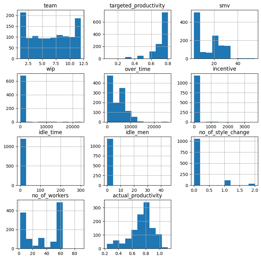

The histograms confirm a few things we suspected. idle_time and idle_men show virtually no variation, with bars only at zero. Let's count the non-zero values:

print(len(df[(df["idle_time"] > 0)]))
print(len(df[(df["idle_men"] > 0)]))

18
18

Only 18 non-zero values out of 1,197 rows for each of these columns. They carry almost no information and can be dropped.

Learning Insight: Histograms are one of the fastest ways to spot low-variance or near-constant columns. If a column has almost all its values at zero with a tiny bar elsewhere, it's usually not going to help your model learn anything meaningful.

Data Cleaning

Now we'll address everything we found during exploration. Let's fix the department column first:

df.loc[df["department"] == "finishing ", "department"] = "finishing"
df.loc[df["department"] == "sweing", "department"] = "sewing"
df["department"].value_counts()

department
sewing       691
finishing    506
Name: count, dtype: int64

Two clean departments. Now let's drop the columns we won't be using:

# removing date column (due to short time frame, probably not useful for our model)
# removing idle_time and idle_men due to few non-zero values
# removing wip due to many null values
# removing no_of_style_change due to few non-zero values
df = df.drop(["date", "idle_time", "idle_men", "wip", "no_of_style_change"], axis=1)
df.head(3)

    quarter department       day  team  targeted_productivity    smv  over_time  incentive  no_of_workers  actual_productivity
0  Quarter1     sewing  Thursday     8                   0.80  26.16       7080         98             59             0.940725
1  Quarter1   finishing  Thursday     1                   0.75   3.94        960          0              8             0.886500
2  Quarter1     sewing  Thursday    11                   0.80  11.41       3660         50             30             0.800570

Next, we'll merge Quarter5 into Quarter4 and convert the quarter labels to integers:

df.loc[df["quarter"] == "Quarter5", "quarter"] = "Quarter4"
df["quarter"].value_counts()

quarter
Quarter1    360
Quarter2    335
Quarter4    292
Quarter3    210
Name: count, dtype: int64

df.loc[df["quarter"] == "Quarter1", "quarter"] = 1
df.loc[df["quarter"] == "Quarter2", "quarter"] = 2
df.loc[df["quarter"] == "Quarter3", "quarter"] = 3
df.loc[df["quarter"] == "Quarter4", "quarter"] = 4
df["quarter"] = df["quarter"].astype("int")

Learning Insight: After doing a .value_counts() on the quarter column, the output may appear to show integers, but the underlying dtype is still a string. Always follow up with .astype() to make sure the conversion actually took effect in the dataframe. It's an easy gotcha to miss.

Now let's fix the no_of_workers column, which is currently stored as a float:

# number of workers is currently a float, but can't have a fraction of a worker. convert to int
df["no_of_workers"] = df["no_of_workers"].astype("int")

And round actual_productivity to two decimal places, matching the precision of targeted_productivity:

df["actual_productivity"] = df["actual_productivity"].round(2)
df.head(2)

   quarter department       day  team  targeted_productivity    smv  over_time  incentive  no_of_workers  actual_productivity
0        1     sewing  Thursday     8                   0.80  26.16       7080         98             59                 0.94
1        1   finishing  Thursday     1                   0.75   3.94        960          0              8                 0.89

Now we can create our classification target. A day is productive if actual_productivity meets or exceeds targeted_productivity:

# setting new column for classifier based on whether targeted productivity was reached
df["productive"] = df["actual_productivity"] >= df["targeted_productivity"]
df.sample(10, random_state=14)

     quarter  dept_sewing        day  team  targeted_productivity    smv  over_time  incentive  no_of_workers  actual_productivity  productive
959        4            0   Thursday    10                   0.70   2.90       3360          0              8                 0.41       False
464        4            0   Tuesday     8                   0.65   3.94        960          0              8                 0.85        True
672        2            1    Sunday     7                   0.70  24.26       6960          0             58                 0.36       False
...

We can spot-check the logic: row 959 has actual_productivity of 0.41 against a target of 0.70, so productive is False. Looks correct.

Preparing Data for Machine Learning

Decision trees need numeric inputs only. We have three remaining categorical columns to address: department, quarter, and day. We'll also need to handle team, since it's a numeric identifier, not a meaningful number.

Let's start with department. Since it has only two values, we can convert it to a binary column:

# convert department column to boolean
df = df.rename(columns={"department": "dept_sewing"})
df["dept_sewing"] = df["dept_sewing"].map({"finishing": 0, "sewing": 1}).astype("int64")
df.head(10)

   quarter  dept_sewing       day  team  targeted_productivity    smv  over_time  incentive  no_of_workers  actual_productivity  productive
0        1            1  Thursday     8                   0.80  26.16       7080         98             59                 0.94        True
1        1            0  Thursday     1                   0.75   3.94        960          0              8                 0.89        True
...

For quarter, day, and team, the numeric values are labels, not quantities. Quarter 4 isn't four times Quarter 1, and Team 12 isn't "more" than Team 6. We'll convert each with pd.get_dummies() to create proper binary columns:

# make quarter column into dummies (numeric order is *not* actually part of these values so they should be categorical)
df = pd.concat([df, pd.get_dummies(df["quarter"], prefix="q")], axis=1).drop(["quarter"], axis=1)

# day column to dummies
df = pd.concat([df, pd.get_dummies(df["day"], prefix=None)], axis=1).drop(["day"], axis=1)

# team column to dummies
df = pd.concat([df, pd.get_dummies(df["team"], prefix="team")], axis=1).drop(["team"], axis=1)
df.sample(10, random_state=14)

     dept_sewing  targeted_productivity    smv  over_time  incentive  no_of_workers  actual_productivity  productive   q_1   q_2  ...  team_10  team_11  team_12
959            0                   0.70   2.90       3360          0              8                 0.41       False  False  False  ...     True    False    False
464            0                   0.65   3.94        960          0              8                 0.85        True  False  False  ...    False    False    False
...

10 rows × 30 columns

Everything is numeric now. True and False values are treated as 1 and 0 under the hood, so the model can work with them directly. We're ready to build.

Learning Insight: One of the most common mistakes when preparing data for decision trees is leaving numeric-looking identifiers (like team numbers) as raw integers. The model will treat them as continuous values with order and magnitude, which introduces false relationships. Always ask: does a higher value here actually mean "more" of something?

Building the Decision Tree

Let's import our modeling tools and split the data:

from sklearn.model_selection import train_test_split
from sklearn.tree import DecisionTreeClassifier
from sklearn.tree import plot_tree

# Feature and target columns
X = df.drop(["actual_productivity", "productive"], axis=1)
y = df["productive"]

X_train, X_test, y_train, y_test = train_test_split(X, y, test_size=0.2, shuffle=True, random_state=24)

We drop both actual_productivity and productive from X — the model can't see the raw productivity numbers it used to calculate the target, or it would be cheating. We use shuffle=True because the data is sorted by date, and we don't want the training and test splits to come from different time periods.

Now let's instantiate and train the tree:

tree = DecisionTreeClassifier(max_depth=3, random_state=24)
tree.fit(X_train, y_train)

Two lines of code, and a trained decision tree. Let's get some predictions from it:

y_pred = tree.predict(X_test)

Learning Insight: We set max_depth=3, meaning the tree will ask at most 3 questions before reaching a prediction. This is intentional. A deeper tree will memorize the training data rather than learn patterns from it — this is called overfitting. Think of it like a student who memorizes exact exam answers instead of understanding the material. They'll do great on that test, but fail any question they haven't seen before. Keeping depth modest produces a model that generalizes well to new data.

Visualizing and Evaluating the Tree

Let's check accuracy on our held-out test data first:

from sklearn.metrics import accuracy_score
print("Accuracy:", round(accuracy_score(y_test, y_pred), 2))

Accuracy: 0.85

85% accuracy. For a dataset this noisy and with this level of preprocessing, that's a strong result. Now let's see the tree itself:

plt.figure(figsize=[20.0, 8.0])
_ = plot_tree(tree,
              feature_names=X.columns,
              class_names=["Unproductive", "Productive"],
              filled=True,
              rounded=False,
              proportion=True,
              fontsize=11)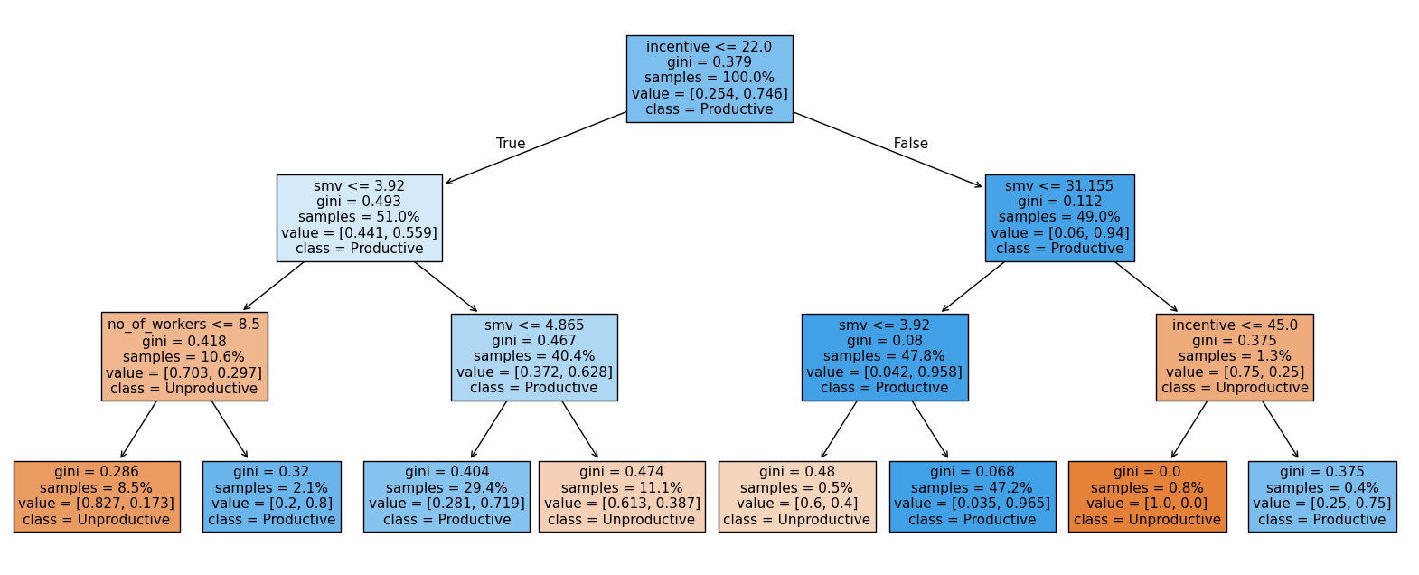

This is one of the best things about decision trees: the model is human-readable. Let's walk through what it's telling us.

Start at the root of the tree. The first question is whether incentive is greater than 22. If it is, we move to the right side of the tree, where the model already shows a strong lean toward Productive days.

Next, the tree asks whether smv is less than or equal to 31.155. Almost all of this group continues down the left branch, where the model then checks whether smv is greater than 3.92.

This final split leads to the largest leaf in the entire tree, covering 47.2% of the dataset. These days are classified as Productive, with a very low Gini impurity (0.068). That low impurity tells us the model is very confident in this prediction.

In practical terms, the clearest pattern in the data is this: when incentives are above 22 and task times fall in a moderate range (not extremely low), the day is very likely to be productive. This combination stands out as the strongest and most consistent signal in the model.

Learning Insight: The fact that incentive and smv (Standard Minute Value) dominate the tree is a meaningful business finding. Incentive showing up as the root node suggests that whether or not a financial reward is offered is the single strongest driver of whether a day hits its productivity target. That's a direct, actionable insight for factory management.

Understanding the Node Information

Each box in the tree shows four pieces of information:

The question being asked at that node
Gini: a measure of impurity. Values closer to 0 mean the node contains mostly one class (more predictive). Values closer to 0.5 mean the classes are evenly mixed.
Samples: the proportion of the dataset represented at that node
Class: what the model would predict if it stopped here

Confusion Matrix

Accuracy alone doesn't tell the full story. Let's look at where the model makes mistakes:

from sklearn.metrics import confusion_matrix
confusion_matrix(y_test, y_pred)

array([[ 35,  24],
       [ 13, 168]])

Reading the confusion matrix:

True Negatives (top-left, 35): Days correctly predicted as unproductive
False Positives (top-right, 24): Days predicted as productive but were actually unproductive
False Negatives (bottom-left, 13): Days predicted as unproductive but were actually productive
True Positives (bottom-right, 168): Days correctly predicted as productive

The model is more likely to misclassify an unproductive day as productive (24 cases) than the reverse (13 cases). In a factory context, this means management might occasionally plan around an expected productive day that doesn't deliver. Worth flagging to stakeholders.

Precision, Recall, and F1

from sklearn.metrics import precision_score, recall_score, f1_score

print("Precision:", round(precision_score(y_test, y_pred), 2))
print("Recall:", round(recall_score(y_test, y_pred), 2))
print("F1 Score:", round(f1_score(y_test, y_pred), 2))
print("----")
print("Accuracy:", round(tree.score(X_test, y_test), 2))

Precision: 0.88
Recall: 0.93
F1 Score: 0.9
----
Accuracy: 0.85

All metrics are clustering near 90%, which is a good sign that the model is performing consistently rather than excelling on one type of prediction while failing on another. Precision of 0.88 means that when the model predicts "productive," it's right 88% of the time. Recall of 0.93 means it catches 93% of the days that were actually productive.

Cross-Validation

To make sure our results hold up across different data splits and aren't just a lucky test set, let's run 10-fold cross-validation:

from sklearn.model_selection import cross_val_score

scores = cross_val_score(tree, X, y, cv=10)
print("Cross Validation Accuracy Scores:", scores.round(2))
print("Mean Cross Validation Score:", scores.mean().round(2))

Cross Validation Accuracy Scores: [0.85 0.88 0.81 0.87 0.87 0.82 0.72 0.76 0.84 0.79]
Mean Cross Validation Score: 0.82

The mean drops slightly to 0.82, but that's expected since cross-validation is a more rigorous test. The lowest single fold scored 0.72 — still reasonable. We can also check precision, recall, and F1 across all 10 folds:

from sklearn.model_selection import cross_validate

multiple_cross_scores = cross_validate(tree, X, y, cv=10,
                                       scoring=("precision", "recall", "f1"))

print("Mean Cross Validated Precision:", round(multiple_cross_scores["test_precision"].mean(), 2))
print("Mean Cross Validated recall:", round(multiple_cross_scores["test_recall"].mean(), 2))
print("Mean Cross Validated F1:", round(multiple_cross_scores["test_f1"].mean(), 2))

Mean Cross Validated Precision: 0.85
Mean Cross Validated recall: 0.92
Mean Cross Validated F1: 0.88

Solid and consistent across the board.

Learning Insight: Cross-validation is essentially running the same experiment 10 times with different data configurations. If your model only performs well on one specific split, that's a red flag. Seeing consistent performance across all 10 folds is what gives us confidence to present these results to stakeholders.

Validating with a Random Forest

One more check. A random forest builds 100 different decision trees, each on a slightly different sample of the data, and combines their predictions. If our single tree is genuinely learning good patterns, the forest should confirm it:

from sklearn.ensemble import RandomForestClassifier

forest = RandomForestClassifier(oob_score=True, random_state=24)
forest.fit(X_train, y_train)

y_pred_forest = forest.predict(X_test)
print("Accuracy:", round(accuracy_score(y_test, y_pred_forest), 2))

Accuracy: 0.85

print("Out Of Bag Score:", round(forest.oob_score_, 2))

Out Of Bag Score: 0.83

The random forest matches our single tree at 85% accuracy on the test set, and scores 0.83 on the out-of-bag estimate (a built-in cross-validation method unique to random forests). This is strong corroboration that our depth-3 decision tree is capturing real patterns, not just memorizing the training data.

Learning Insight: The out-of-bag (OOB) score is a free cross-validation check you get with random forests. Each tree is trained on a different bootstrap sample, meaning some data points are left out of every individual tree's training. Those left-out points are used to evaluate that tree. The OOB score aggregates these evaluations across all 100 trees, giving you a reliable estimate of generalization performance without needing a separate validation split.

Key Takeaways

Walking through this project, a few things stand out:

Incentive and task time are the dominant drivers of productivity. The decision tree asks about incentive and smv at nearly every branch. For factory management, this is actionable: financial incentives and realistic task time allocation appear to be the levers most worth pulling.

Decision trees are powerful communication tools. Unlike most machine learning models, a shallow decision tree can be shown directly to non-technical stakeholders. You can walk a factory manager through the exact logic the model uses, question by question.

Multiple evaluation metrics matter. Our accuracy was 85%, but the confusion matrix showed us that the model's errors lean toward false positives — predicting productivity that doesn't materialize. That nuance matters for how the business uses the predictions.

A single tree backed by a random forest is a trustworthy result. When your 10-fold cross-validation and a 100-tree ensemble both confirm your single model's accuracy, you can present those findings with confidence.

Next Steps

There are several directions worth exploring from here:

Try a regression tree instead. Rather than predicting productive vs. unproductive, predict the actual productivity value directly. Most of the data preparation work is already done — the main change is your target variable and model type.

Add productivity tiers. Instead of a binary target, consider creating multi-class categories like "insufficient," "satisfactory," and "exceeds target." This gives stakeholders more granular predictions to act on.

Keep wip in the dataset. Work in Progress was dropped due to missing values, but it could be a meaningful predictor. Try imputing the missing values and see whether including wip improves performance.

Investigate the age bands in the data. The dataset covers only three months, and date was dropped early. It's worth exploring whether productivity patterns shift over time, or whether certain teams or quarters behave differently enough to warrant separate models.

Sharing Your Work

When you complete this project, consider sharing it on GitHub as a Jupyter notebook. Include Markdown cells that explain your reasoning at each step — especially why you dropped certain columns, how you handled the Quarter5 issue, and what the decision tree visualization means in plain language. A notebook with clear explanations is far more impressive to employers than one that's just code.

If you get stuck or want to discuss your results, tag @Anna_strahl in the Dataquest Community. And if you're looking to build a stronger foundation before tackling this project, the Decision Tree and Random Forest Modeling in Python course covers the core concepts we applied here.

Happy modeling!

Project Tutorial: Predicting Employee Productivity with Decision Trees and Random Forests

What You'll Learn

Before You Start

Setting Up Your Environment

Exploratory Data Analysis (EDA)

Data Cleaning

Preparing Data for Machine Learning

Building the Decision Tree

Visualizing and Evaluating the Tree

Understanding the Node Information

Confusion Matrix

Precision, Recall, and F1

Cross-Validation

Validating with a Random Forest

Key Takeaways

Next Steps

Sharing Your Work

Project Tutorial: Profitable App Profiles for the App Store and Google Play Markets

Project Tutorial: Build a Python Word Guessing Game

Project Tutorial: Predicting Employee Productivity with Decision Trees and Random Forests

What You'll Learn

Before You Start

Setting Up Your Environment

Exploratory Data Analysis (EDA)

Data Cleaning

Preparing Data for Machine Learning

Building the Decision Tree

Visualizing and Evaluating the Tree

Understanding the Node Information

Confusion Matrix

Precision, Recall, and F1

Cross-Validation

Validating with a Random Forest

Key Takeaways

Next Steps

Sharing Your Work

More learning resources

Project Tutorial: Profitable App Profiles for the App Store and Google Play Markets

Project Tutorial: Build a Python Word Guessing Game