An Intro to Logistic Regression in Python (w/ 100+ Code Examples)

The logistic regression algorithm is a probabilistic machine learning algorithm used for classification tasks. This is usually the first classification algorithm you'll try a classification task on. Unlike many machine learning algorithms that seem to be a black box, the logisitc regression algorithm is easily understood.

In this tutorial, you'll learn everything you need to know about the logistic regression algorithm. You'll start by creating a custom logistic regresssion algorithm. This will help you understand everything happening under the hood and how to debug problems with your logisitic regression models. Next, you'll learn how to train and optimize Scikit-Learn implementation of the logistic regression algorithm. Finally, you'll learn how to handle multiclass classification tasks with this algorithm.

This tutorial covers L1 and L2 regularization, hyperparameter tuning using grid search, automating machine learning workflow with pipeline, one vs rest classifier, object-oriented programming, modular programming, and documenting Python modules with docstring.

---

Build Your Own Custom Logistic Regression Model

In this section, you'll build your own custom logistic regression model using stochastic gradient descent. This logistic regression algorithm can be trained with batch, mini-batch, or stochastic gradient descent.

In batch gradient descent, the entire train set is used to update the model parameters after one epoch. For a very large train set, it may be best to update the model parameters with a random subset of the data, as training the model with the whole set would be computationally expensive. This is the idea behind mini-batch gradient descent. In stochastic gradient descent, model parameters are updated after training on every single data point in the train set. This method can be used when the train set is small.

To summarize, let assume that we have a train set with m rows. The batch size, n, used to train and update model parameters for:

• batch gradient descent: $n = m$
• mini-batch gradient descent: $1 < n < m$
• stochastic gradient descent: $n = 1$

The number of rows, m, in our train set is small. It is okay to use stochastic gradient descent for our example. Next, let's discuss the methods in our custom logistic regression model.

The __init__ Method

To create an instance of an object, you need to initialize or assign some starting values. These starting values are passed through the __init__ method. To create an instance of our Stochastic Logistic Regression (SLR) class, we have to pass the learning_rate, n_epochs, and cutoff parameters.

In addition, we have also initialized our intercept, b, and coefficients w values. These are the values that we want to optimize using gradient descent.

class SLR(object):
    """
    This is the SLR class
    """
def __init__(self, learning_rate=10e-3, n_epochs=10_000, cutoff=0.5):
        """
        The __init__ method
        Params:
            learning_rate
            n_epochs
            cutoff
        """
        self.learning_rate = learning_rate  
        self.n_epochs = n_epochs   
        self.cutoff = cutoff

        self.w = None
        self.b = 0.0

The __repr__ Method

The __repr__ method helps us make our own printable representation of an object. To understand how this works, let's print the SLR class without the __repr__ method:

Create an instance of the SLR class

slr0 = SLR()

Print the slr0 object

print(slr0)

When we print the instance of the SLR class without the __repr__ method, the output is the address of the object in memory. With the __repr__ method, we define how we want the object to be printed, as shown below:

class SLR(object):
    ...

    def __init__(self, learning_rate=10e-3, n_epochs=10_000, cutoff=0.5):
        ...

        self.learning_rate = learning_rate  
        self.n_epochs = n_epochs   
        self.cutoff = cutoff

        ...

    def __repr__(self):
        params = {
            'learning_rate': self.learning_rate,
            'n_epochs': self.n_epochs,
            'cutoff': self.cutoff
        }
        return "SLR({0}={3}, {1}={4}, {2}={5})".format(*params.keys(), *params.values())

Create an instance of the SLR class

slr1 = SLR()

Print the slr1 object

print(slr1)

The new instance of our SLR class prints exactly what we have defined in our __repr__ method. We have excluded some things from the SLR class for brevity. We will use ellipsis, ..., to represent the parts where items have been excluded.

The sigmoid Method

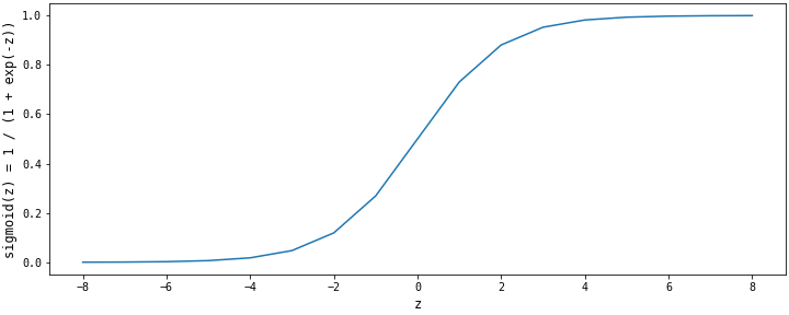
The sigmoid method is at the heart of the logistic regression algorithm. It maps the linear function $z = {w^T}x + b$ to the open interval $(0, 1)$. The sigmod method outputs probability values that we will compare to the cutoff for predictions. It is mathematically represented as: ${\large {1 \over {1 + e^{-z}}}}$

The shape of the sigmoid function is shown in the figure below. The sigmoid function has an asymptote that approaches a value of $1$ when $z$ goes to $+\infty$ and an asymptote that approaches the value of $0$ when $z$ goes to $-\infty$.

class SLR(object):
    ...

    def __init__(self, learning_rate=10e-3, n_epochs=10_000, cutoff=0.5):

        ...

    def __repr__(self):

         ...    

    def sigmoid(self, z):
        """
        The sigmoid method:
        Param:
            z
        Return:
            1.0 / (1.0 + exp(-z))
        """
        return 1.0 / (1.0 + np.exp(-z))

The predict_proba Method

This method predicts the probability value for each row. The value of the linear function, z, is calculated using the intercept, b, and coefficients, w, parameters. The value of z is passed to sigmoid method to get a probabilty value.

class SLR(object):
    ...

    def __init__(self, learning_rate=10e-3, n_epochs=10_000, cutoff=0.5):
        ...

    def __repr__(self):
        ...   

    def sigmoid(self, z):
        ...

    def predict_proba(self, row):
        """
        The predict_proba
        Param:
            row
        Return:
            sigmoid(z)
        """
        z = np.dot(row, self.w) + self.b
        return self.sigmoid(z)

The fit Method

This method implements stochastic gradient descent to update the w and b parameters. One of the first things to do is intialize the parameters of w and b. The value of b is set to 0.0 and the values in w are set to zeros, as shown below:

class SLR(object):
    ...

    def __init__(self, learning_rate=10e-3, n_epochs=10_000, cutoff=0.5):
        ...
        self.w = None
        self.b = 0.0
    ...

    def fit(self, X, y):
        ...

        self.w = np.zeros(X.shape[1]) 

        ...  

The next important steps are to use the values of b and w to calculate a probability value and calculate the gradients with respect to w and b. These are shown mathematically below:

• Calcualte a probability value, yhat: $\hat{y_i}$ = ${\large {1 \over {1 + e^{-z_i}}}}$
• Calculate gradient w.r.t b, grad_b: $\nabla_b = \hat{y_i} - y_i$
• Calculate gradient w.r.t w, grad_w: $\nabla_w = x_i(\hat{y_i} - y_i)$

class SLR(object):
    ...

    def fit(self, X, y):
        ...

        for n_epoch in range(1, self.n_epochs + 1):
            losses = []
            for i in range(self.m):
                # Calculate the probability value for a row
                yhat = self.predict_proba(X[i])
                # Calculate the gradient w.r.t b
                grad_b = yhat - y[i]
                # Calculate the gradient w.r.t w
                grad_w =  X[i] * (yhat - y[i])         

The final steps are to update the values of b and w using the learning rate, $\alpha$, and calculate the loss function:

• Update the value of b: $b = b - \alpha\nabla_b$
• Update the value of w: $w = w - \alpha\nabla_w$
• Calculate log-loss: $-(y_i\log(\hat{y}_i + (1 - y_i)\log((1 - \hat{y}_i))$

class SLR(object):
    ...
    def fit(self, X, y):
        ...

        for n_epoch in range(1, self.n_epochs + 1):
            losses = []
            for i in range(self.m):
                ...        
                # Update the value of w
                self.w -= self.learning_rate * grad_w / self.m
                # Update the value of b
                self.b -= self.learning_rate * grad_b / self.m
                # Calculate the log-loss
                loss = -1/self.m * (y[i] * np.log(yhat) + (1 - y[i]) * np.log(1 - yhat))
                losses.append(loss)
            # Calculate the cost fuction
            self.cost.append(sum(losses))               

After training for one epoch, the cost function is calculated for that epoch. The cost function is the average of the loss function. If you'd like to learn more about gradient descent and how the parameters were derived, read this article on DataQuest.

Putting everything in the fit method together, we get:

class SLR(object):
    ...

    def __init__(self, learning_rate=10e-3, n_epochs=10_000, cutoff=0.5):
        ...

    def __repr__(self):
        ...   

    def sigmoid(self, z):
        ...

    def predict_proba(self, row):
        ...

    def fit(self, X, y):
        """
        The fit method implement stochastic gradient descent
        Param
            X, y
        Return
            None
        """
        if not isinstance(X, np.ndarray):
            X = X.to_numpy()

        if not isinstance(y, np.ndarray):
            y = y.to_numpy()

        self.w = np.zeros(X.shape[1])
        self.cost = []

        self.m = X.shape[0]
        self.log_loss = {}
        self.cost = []

        for n_epoch in range(1, self.n_epochs + 1):
            losses = []
            for i in range(self.m):
                yhat = self.predict_proba(X[i])
                grad_b = yhat - y[i]
                grad_w =  X[i] * (yhat - y[i])

                self.w -= self.learning_rate * grad_w / self.m
                self.b -= self.learning_rate * grad_b / self.m
                loss = -1/self.m * (y[i] * np.log(yhat) + (1 - y[i]) * np.log(1 - yhat))
                losses.append(loss)

            self.cost.append(sum(losses))               

The predict Method

This method is used to make discrete predictions. It uses the predict_proba method to get the probability values, then compares these probability values against a cutoff. Probability values below the cutoff belong to one class, and those greater than or equal to the cutoff belong to another class.

class SLR(object):
    ...

    def __init__(self, learning_rate=10e-3, n_epochs=10_000, cutoff=0.5):
        ...

    def __repr__(self):
        ...    

    def sigmoid(self, z):
        ...

    def predict_proba(self, row):
        ...

    def fit(self, X, y):
        ...

    def predict(self, X):
        if not isinstance(X, np.ndarray):
            X = X.to_numpy()

        self.predict_probas = []
        for i in range(X.shape[0]):
            ypred = self.predict_proba(X[i])
            self.predict_probas.append(ypred)

        return (np.array(self.predict_probas) >= self.cutoff) * 1.0     

The score Method

This method is used to calculate the accuracy score, using the trained parameters of the model. It uses the predict method to make discrete predictions and compare these values against the actual.

class SLR(object):
    ...

    def __init__(self, learning_rate=10e-3, n_epochs=10_000, cutoff=0.5):
        ...

    def __repr__(self):
        ...    

    def sigmoid(self, z):
        ...

    def predict_proba(self, row):
        ...

    def fit(self, X, y):
        ...

    def predict(self, X):
        ...

    def score(self, X, y):
        """
        The score method
        Param
            X, y
        Return
            accuracy_score(y, ypred)
        """
        ypred = self.predict(X)
        y = y.to_numpy()
        return accuracy_score(y, ypred)

The Logistic Regression Module

Putting everything inside a python script (.py file) and saving (slr.py) gives us a custom logistic regression module. You can reuse the code in your logistic regression module by importing it. You can use your custom logistic regression module in multiple Python scripts and Jupyter notebooks.

It's important that you save the module in the same directory with the script or notebook you'll be working on. Let's assume that our slr.py file is saved inside the logreg directory. In the next section, we shall be working with our custom module.

../logreg/slr.py

"""
    # slr.py 
    This is stochastic logistic regression module
    To use:
        from slr import SLR
        # Import the SLR class from the module and use its methods
        log_reg = SLR()      # Initialization with default params
        log_reg.fit(X, y)    # Fit with train set
        log_reg.predict(X)   # Make predictions with test set
        log_reg.score(X,y)   # Get accuracy score

    Method:
        __init__
        __repr__
        sigmoid
        predict
        predict_proba
        fit
        score   
"""
import numpy as np
from sklearn.metrics import accuracy_score

class SLR(object):
    """
    This is the SLR class
    """

    def __init__(self, learning_rate=10e-3, n_epochs=10_000, cutoff=0.5):
        """
        The __init__ method
        Params:
            learning_rate
            n_epochs
            cutoff
        """
        self.learning_rate = learning_rate  
        self.n_epochs = n_epochs   
        self.cutoff = cutoff

        self.w = None
        self.b = 0.0

    def __repr__(self):
        params = {
            'learning_rate': self.learning_rate,
            'n_epochs': self.n_epochs,
            'cutoff': self.cutoff
        }
        return "SLR({0}={3}, {1}={4}, {2}={5})".format(*params.keys(), *params.values())    

    def sigmoid(self, z):
        """
        The sigmoid method:
        Param:
            z
        Return:
            1.0 / (1.0 + exp(-z))
        """
        return 1.0 / (1.0 + np.exp(-z))

    def predict_proba(self, row):
        """
        The predict_proba
        Param:
            row
        Return:
            sigmoid(z)
        """
        z = np.dot(row, self.w) + self.b
        return self.sigmoid(z)

    def predict(self, X):
        if not isinstance(X, np.ndarray):
            X = X.to_numpy()

        self.predict_probas = []
        for i in range(X.shape[0]):
            ypred = self.predict_proba(X[i])
            self.predict_probas.append(ypred)

        return (np.array(self.predict_probas) >= self.cutoff) * 1.0  

    def score(self, X, y):
        """
        The score method
        Param
            X, y
        Return
            accuracy_score(y, ypred)
        """
        ypred = self.predict(X)
        y = y.to_numpy()
        return accuracy_score(y, ypred)

    def fit(self, X, y):
        """
        The fit method implement stochastic gradient descent
        Param
            X, y
        Return
            None
        """
        if not isinstance(X, np.ndarray):
            X = X.to_numpy()

        if not isinstance(y, np.ndarray):
            y = y.to_numpy()

        self.w = np.zeros(X.shape[1])
        self.cost = []

        self.m = X.shape[0]
        self.log_loss = {}
        self.cost = []

        for n_epoch in range(1, self.n_epochs + 1):
            losses = []
            for i in range(self.m):
                yhat = self.predict_proba(X[i])
                grad_b = yhat - y[i]
                grad_w =  X[i] * (yhat - y[i])

                self.w -= self.learning_rate * grad_w / self.m
                self.b -= self.learning_rate * grad_b / self.m
                loss = -1/self.m * (y[i] * np.log(yhat) + (1 - y[i]) * np.log(1 - yhat))
                losses.append(loss)

            self.cost.append(sum(losses))               

---

Working with the slr Module

../logreg/stochastic.ipynb

import slr
from slr import SLR

We've imported the slr module and the SLR class inside this module. Does this step look familiar? Yes! You must've imported several Python libraries in the past--numpy, pandas, and matplotlib are widely used.

You can learn about a Python library, module, class, method, and function from their documentation. Docstrings are an excellent way to document how things work in Python. To view the documentation of an unfamiliar module or function, you can use the __doc__ attribute. You can view the methods and attributes of a Python object with the dir() function.

Attributes and methods of the slr module

dir(slr)

Attributes and methods of the SLR class

dir(SLR)

Both the slr module and SLR class have the __doc__ attribute. We can view what is written in their docstrings:

Docstring in the slr.py module

print(slr.__doc__)

print(SLR.__doc__)

Let's also view the docstrings in the sigmoid and fit methods:

print(SLR.sigmoid.__doc__)

print(SLR.fit.__doc__)

Alternatively, you can view all the docstrings with the help() function:

help(SLR)

---

Understanding Logistic Regression with slr

../logreg/stochastic.ipynb

import numpy as np
import pandas as pd
import matplotlib.pyplot as plt
from sklearn.pipeline import Pipeline
from sklearn.datasets import load_breast_cancer
from sklearn.metrics import classification_report
from sklearn.model_selection import train_test_split
from sklearn.preprocessing import StandardScaler

import warnings
warnings.filterwarnings('ignore')

Load and Split Data

../logreg/stochastic.ipynb

Load data

bin_data = load_breast_cancer()
X = bin_data.data
y = bin_data.target

Store data as pandas objects

X = pd.DataFrame(X, columns=bin_data.feature_names)
y = pd.Series(y, name='diagnosis', dtype=np.int8)

pd.options.display.max_columns = X.shape[1]
X.head()

The target has two classes - binary classification task

y.value_counts()

Split the data into train and test sets

X_train, X_test, y_train, y_test = train_test_split(X, y, train_size=0.75, random_state=47)

Loss and Cost Functions for Logistic Regression

The linear regression algorithm uses the mean squared error cost function. This cost function is always convex for a linear function $z = {w^T}x + b$. In other words, the cost function always approaches its global minimum during training.

The logistic regression algorithm uses the sigmoid function, which is exponential. This function isn't always convex with the mean squared error cost function. Thus, our logistic regression can get stuck in a local minimum. We have to randomly initialize our model and train several to be sure that we are getting the best results.

We initialized our weights to zeros while building the SLR because we are using a cost function that is always convex with the sigmoid function. Otherwise we should have randomly intialized our weights if we were using the mean squared error cost function.

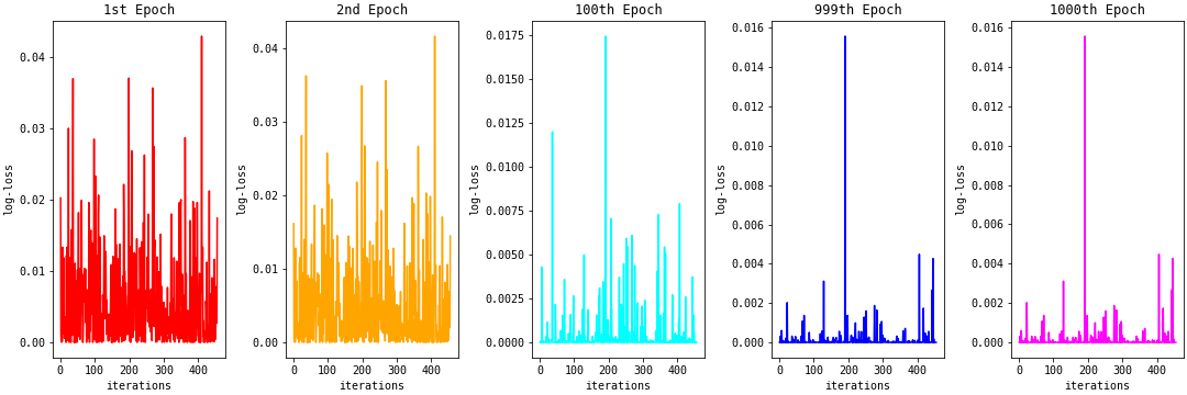
The loss function used for training the logistic regression algorithm is called log-loss. It is given mathematically as:

• log-loss = $-y_i \cdot \log\hat{y} - (1 - y_i) \cdot \log(1 - \hat{y})$.

The cost function, $J(w, b)$, is just the average of the log-loss function for an epoch:

• $J(w, b) = -{1 \over m}\sum^m_{i=1}y_i \cdot \log\hat{y} + (1 - y_i) \cdot \log(1 - \hat{y}) $

The figure below shows the log-loss plot for each row in the train set for the 1st, 2nd, 100th 999th, and 1000th epochs. There are many spikes in log-loss values in the 1st epoch. As we continue to train, the spikes reduce, and we have many log-loss values closer to zero in the 1000th epoch.

When we average the log-loss values for each epoch, we get the cost function. We expect the cost function value to decrease as the number of epochs increases. The cost function plot when we average the log-loss values for the above examples is shown below:

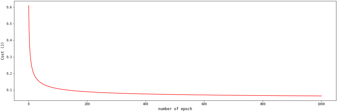
The above cost function plot is convex. The cost function value continues to approach the global minimum. If you're interested in learning more about convexity and the log-loss function, this article explains why the log-loss function works for logistic regression, but the mean squared error doesn't. While this exchange tries to prove that the log-loss function is always convex.

Next, let's look at how the learning rate affects the shape of the cost function.

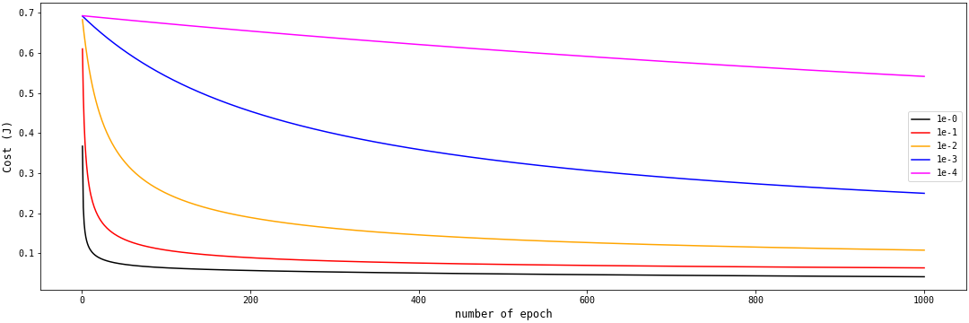
Cost Function and Learning Rate

The learning rate is an important parameter in our SLR model. Here, we created five instances of the SLR class with different learning rates. When the learning rate was very small, the cost function, $Cost (J)$, was a straight horizontal line.

As we increase the learning rate from ${10^{-4}}$ to $10^{-0}$, we get the first half of a U-shaped curve. The larger the learning rate, the faster the cost function approaches the global minimum.

Do you think we should continue to increase the learning rate? There are issues with the model when the learning rate is greater than 1. When we create an instance of the SLR class with a learning rate of 4, we get the plot on Part A in the figure below:

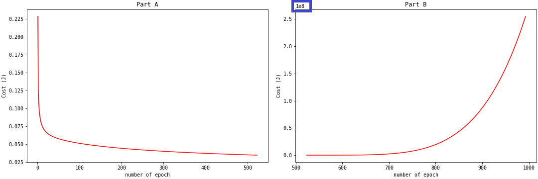
What happened to the cost function after 500 epochs? The predict_proba method started to output probabilities very close to zero. The log-loss (and by extension, the cost function) values become positive infinity. You will get np.nan for np.inf log-loss values. This is what happened after 500 epochs. We weren't able to make a plot of the cost function after this point. If you want to observe these np.inf values, you can use the np.nan_to_num function on your log-loss: np.nan_to_num(log-loss). This function replaces np.inf with very large values.

With a very large learning rate, the cost function misses the global minimum by jumping from Part A to larger values, like in Part B. Thus, it is important that we choose the appropriate learning rate.

---

The Performance of the slr

In this section, we'll train and make predictions with our custom logistic regression model. First, let's identify a baseline for our model.

Baseline Model

y_train.value_counts(normalize='True')

y_test.value_counts(normalize='True')

If we predict 1 for all the entries in the train and test set, we get an accuracy of 63% and 61%, respectively. Thus, 63% is the baseline for our train set. It is 61% for the test set. We expect our custom model to outperform the baseline.

Scale Features

X_train.describe()

X_train.info()

The describe() and info() methods tell us that the features in our data are continuous variables on different scales. Before training, we'll first scale the features with the StandardScaler() function. We don't want to do this manually, so we'll connect the scaling and fitting using a Pipeline:

Train the SLR

Connect StandardScaler() and SLR() with a pipe

pipe0 = Pipeline([
    ('scaler', StandardScaler()),
    ('lr', SLR(learning_rate=1e-2, n_epochs=1000, cutoff=0.5))
])

Train the model

pipe0.fit(X_train, y_train)

Get the accuracies of the train and test set

Check if they beat the baseline model

accuracies = {
    'train accuracy': pipe0.score(X_train, y_train), 
    'test accuracy': pipe0.score(X_test, y_test)
}

print(*accuracies.items())

Check other classification metrics for test set

print(classification_report(y_test, pipe0.predict(X_test)))

Check other classification metrics for train set

print(classification_report(y_train, pipe0.predict(X_train)))

Our custom slr model outperformed the baseline on the train and test sets. This is so cool!

Next, let's investigate whether the cutoff value significantly affects prediction accuracies.

Predict with the slr

We will make predictions with pipe0 in this section. Then we'll plot the predicted probabilities using a cutoff of 0.5. Points above the cutoff belong in one class, and points below the cutoff belong in a separate class.

import matplotlib
matplotlib.rcParams['font.family'] = 'monospace'

Predict with pipe0

predictions = pipe0.predict(X_test)
predict_probas = pipe0['lr'].predict_probas
cutoff = pipe0['lr'].cutoff

Plot predicted probabilities

fig = plt.figure(figsize=(15, 5), constrained_layout=True)
x = range(1, len(predict_probas) + 1)
plt.scatter(x, predict_probas, c=predictions, label='predicted probabilities')
plt.plot(x, [cutoff] * len(predictions), color='red', label='cutoff=0.5')

plt.ylabel('Predicted probabilites', fontsize=12)
plt.xlabel('test data', fontsize=12)
plt.legend(loc=7);

Recall the accuracy values using pipe0

print(*accuracies.items())

We can see from the above plots that there are values close to the cutoff point. Let's assume that these values were among the mis-classified. Let's reduce the cutoff value to 0.35 and observe for improvement:

create a new instance, pipe1, with a cutoff value of 0.35

pipe1 = Pipeline([
    ('scaler', StandardScaler()),
    ('lr', SLR(learning_rate=1e-2, n_epochs=1000, cutoff=0.35))
])

fit pipe1 instance

pipe1.fit(X_train, y_train)

Get predicted probabilities for pipe1

predictions = pipe1.predict(X_test)
predict_probas = pipe1['lr'].predict_probas
cutoff = pipe1['lr'].cutoff

Plot the predicted probabilities

fig = plt.figure(figsize=(15, 5), constrained_layout=True)
x = range(1, len(predict_probas) + 1)
plt.scatter(x, predict_probas, c=predictions, label='predicted probabilities')
plt.plot(x, [cutoff] * len(predictions), color='red', label='cutoff=0.35')

plt.ylabel('Predicted probabilites', fontsize=12)
plt.xlabel('test data', fontsize=12)
plt.legend(loc=5);

Get pipe1 accuracies

accuracies1 = {
    'train accuracy': pipe1.score(X_train, y_train), 
    'test accuracy': pipe1.score(X_test, y_test)
}

print(*accuracies1.items())

Although our accuracies did not improve, we've learned that we can either increase or decrease our cutoff value from the default, depending on the type of problem we are faced with.

Our custom logistic regression model did not perform badly. But we can do much more with the Scikit-Learn implementation of the logistic regression algorithm. This machine learning framework has more features and has been rigorously tested. We'll be using Scikit-Learn going forward.

---

Scikit-Learn Logistic Regression Model

In this section, we'll use the features of the Scikit-Learn logistic regression model. First, we'll train a logistic regression model with no regularization. Then we'll train models with L1, L2, and L1 and L2 regularization.

Let's import this model from Scikit-Learn:

from sklearn.linear_model import LogisticRegression

Without Regularization

Training without regularization simply means setting the penalty parameter to none:

Train sklearn logistic regression model with no regularization: pipe2

pipe2 = Pipeline([
    ('scaler', StandardScaler()),
    ('lr', LogisticRegression(penalty='none'))
])

fit the model

pipe2.fit(X_train, y_train)

Fet model accuracies

accuracies2 = {
    'train accuracy': pipe2.score(X_train, y_train), 
    'test accuracy': pipe2.score(X_test, y_test)
}

print(*accuracies2.items())

We can see that the model is overfitting the train set. The difference between the train and test accuracies is 12%. The purpose of regularization is to prevent overfitting.

Next, let's use the L1 regularization.

With L1 Regularization

Regularization is the modification we make to machine learning algorithms to reduce their generalization errors. In other words, regularization helps us improve a machine learning model's performance on data it hasn't seen before/wasn't trained on.

Regularization in logistic regression simply means adding a regularization parameter to our cost function:

• $J(w, b) = -{1 \over m}\sum^m_{i=1}y_i \cdot \log\hat{y} + (1 - y_i) \cdot \log(1 - \hat{y}) + {\lambda \over m}R(w_i)$

The parameter $\lambda$ and $R(w_i)$ are the regularization parameter and regularization function, respectively. For logistic regression, the regularization parameter, $C$, is given as: $C = {1 \over \lambda}$. For L1 regularization, $R(wi)$ is given as $\sum{j=1}^p|w_i|$.

The logistic regression cost function with L1 regularization becomes:

• $J(w, b) = -{1 \over m}\sum^m_{i=1}y_i \cdot \log\hat{y} + (1 - yi) \cdot \log(1 - \hat{y}) + {1 \over m \cdot C} \sum{j=1}^p|w_i|$

Recall that $w$ is our model's coefficients. Therefore $|w_i|$ is the absolute value of the coefficients.

Next, we are going to implement the Scikit-Learn logistic regression model with L1 regularization. Before then, let's discuss the pros and cons of L1 regularization. The major advantage of the L1 regularization is that it's used for feature selection. The weights of unimportant features are set to zero. Only the coefficients of important features are left. The disadvantage of the L1 regularization is that is does not use statistical techniques to remove features that are collinear. It may remove the most predictive feature from the model out of two collinear features.

We'll use solver='saga' because the saga solver works on all types of penalties or regularization.

Logistic regression with L1 regularization with regularization parameter C=1e-1

pipe3 = Pipeline([
    ('scaler', StandardScaler()),
    ('lr', LogisticRegression(penalty='l1', C=1e-1, solver='saga'))
])

fit the pipe

pipe3.fit(X_train, y_train)

Get the accuracies

accuracies3 = {
    'train accuracy': pipe3.score(X_train, y_train), 
    'test accuracy': pipe3.score(X_test, y_test)
}

print(*accuracies3.items())

Recall that the logistic regression set coefficients to zero. Let's inspect these coefficients from our model below:

df_coefficients = pd.DataFrame(
    {
        'feature': X_train.columns,
        'coefficient': pipe3['lr'].coef_[0]
    }
)

df_coefficients

Let's inspect only the important features below:

(
    df_coefficients[df_coefficients.coefficient != 0]
    .sort_values(by=['coefficient'])
)

Out of the 30 features in our data, only a handful were considered important by the L1 regularization. Next, let's see how L2 regularization works with logistic regression.

With L2 Regularization

For L2 regularization, $R(wi)$ is given as ${1 \over 2}\sum{j=1}^pw_i^2$.

The logistic regression cost function with L2 regularization becomes:

• $J(w, b) = -{1 \over m}\sum^m_{i=1}y_i \cdot \log\hat{y} + (1 - yi) \cdot \log(1 - \hat{y}) + {1 \over 2 \cdot m \cdot C} \sum{j=1}^pw_i^2$

Where $w_i^2$ is the square of the model's coefficients.

The L2 regularization can't perform feature selection, but it's used to prevent overfitting. Logistic regression with L2 regularization is implemented below:

Logistic regression with L2 regularization with regularization parameter C=1e-1

pipe4 = Pipeline([
    ('scaler', StandardScaler()),
    ('lr', LogisticRegression(penalty='l2', C=1e-1, solver='saga'))
])

fit the pipe

pipe4.fit(X_train, y_train)

Get the accuracies

accuracies4 = {
    'train accuracy': pipe4.score(X_train, y_train), 
    'test accuracy': pipe4.score(X_test, y_test)
}

print(*accuracies4.items())

We can observe from the dataframe below that no features have zero coefficients. If we want a simpler model with fewer features, L2 regularization isn't very helpful.

pd.DataFrame(
    {
        'feature': X_train.columns,
        'coefficient': pipe4['lr'].coef_[0]
    }
).sort_values(by=['coefficient'])

With L1 and L2 Regularization

The logistic regression with L1 and L2 regularization uses the L1 and L2 regularization functions. This regularization is called elasticnet and is given mathematically below:

• $J(w, b) = -{1 \over m}\sum^m_{i=1}y_i \cdot \log\hat{y} + (1 - yi) \cdot \log(1 - \hat{y}) + {1 \over m \cdot C} \sum{j=1}^p(\beta \cdot |w_i| + {1 \over 2} \cdot (1 - \beta) \cdot w_i^2)$

The parameter $\beta$ is known as the L1_ratio. It's the mixing effect that L1 and L2 regularization have on the model's coefficients. When this parameter is set to zero, it's L2 regularization. When it's set to 1, it is L1 regularization.

This regularization is implemented below:

Logistic regression with L1 and L2 regularization with regularization parameter C=1e-1 and L1_ratio=0.5

pipe5 = Pipeline([
    ('scaler', StandardScaler()),
    ('lr', LogisticRegression(penalty='elasticnet', l1_ratio=0.5, C=1e-1, solver='saga'))
])

Fit the pipe

pipe5.fit(X_train, y_train)

Get the accuracies

accuracies5 = {
    'train accuracy': pipe5.score(X_train, y_train), 
    'test accuracy': pipe5.score(X_test, y_test)
}

print(*accuracies5.items())

Get the features coefficients

pd.DataFrame(
    {
        'feature': X_train.columns,
        'coefficient': pipe5['lr'].coef_[0]
    }
)

Percentage features for which coefficients are set to zero and those not set to zero

(
    pd.DataFrame(
    {
        'feature': X_train.columns,
        'coefficient': pipe5['lr'].coef_[0]
    })
    .coefficient
    .apply(lambda x: x == 0)
    .value_counts(normalize=True)
)

We have used elasticnet regularization with 50 percent L1_ratio. L1 and L2 regularization have an equal effect on the model coefficients. With this regularization, we've got more important features than using L1 regularization alone.

We haven't attempted to tune the hyperparameters of our model. Let's see how we can optimize model hyperparameters in the following section.

Hyperparameter Tuning with GridSearch

Hyperparameters are the assumptions we explicitly make to control the learning process. If we assume that the learning rate and regularization constant take specific values, we aren't quite sure if these values are actually the optimum.

To find the optimum hyperparameters for our model, we can list a range of values for them. Grid search creates a combination of these parameters and plots them into grids. Our estimator trains on each grid and records the score for the selected metric. If accuracy is the selected metric, grid search select the parameters from the grid that gives the highest accuracy as the best estimator.

Let's assume that we want to optimize a model with C and LR hyperparameters. The listed C values are [1e-1, 1e-3], and those for LR are [2e-1, 2e-3]. Grid search will train on and evaluate the accuracy of each of the grids shown below. The one with the highest accuracy is selected as the best estimator.

You can use grid search for more than two entries in a hyperparamter and for more than two hyperparameters. If three hyperparameters are used, we get a cubiod shape instead of a plane.

Let's optimize our logistic regression model using grid search.

import gridsearchcv

from sklearn.model_selection import GridSearchCV

create pipe - estimator

pipe6 = Pipeline([
    ('scaler', StandardScaler()),
    ('lr', LogisticRegression(solver='saga'))
])

specify hyperparameters and their values

params = {
    'lr__C': [1.0, 1e-1, 1e-2, 1e-3],
    'lr__penalty': ['l1', 'l2', 'elasticnet'],
    'lr__l1_ratio': [0.25, 0.5, 0.75]
}

fit gridsearch with pipe as estimator

grid_pipe6 = GridSearchCV(
    pipe6,
    params,
    cv=5
)

grid_pipe6.fit(X_train, y_train)

get best hyperparameter values

print(grid_pipe6.best_params_)

get the best estimator / model

print(grid_pipe6.best_estimator_)

Explore the best estimator parameter dictionary

grid_pipe6.best_estimator_.get_params()

Get best estimator accuracies

accuracies6 = {
    'train accuracy': grid_pipe6.score(X_train, y_train), 
    'test accuracy': grid_pipe6.score(X_test, y_test)
}

print(*accuracies6.items())

We tuned the hyperparameters to get the highest accuracies for the train and test sets in this tutorial. Maybe we can get even better accuracies if we search outside our current listed values. For example, if our highest listed parameter came out as the best, we may want list more parameter values with the best parameters at the centre of the list. By doing this, we can explore the edges for better parameters.

Next, we'll see how to handle multiclass classification with the logistic regression model.

---

Mutliclass Classification with Logistic Regression

Load Multiclass Data

from sklearn.datasets import load_wine

mult_data = load_wine()
X = mult_data.data
y = mult_data.target

X = pd.DataFrame(X, columns=mult_data.feature_names)
y = pd.Series(y, name='class', dtype=np.int8)

X_train, X_test, y_train, y_test = train_test_split(X, y, train_size=0.75, random_state=47)

X_train.head()

Baseline Model

get baseline for train set

y_train.value_counts(normalize=True)

get baseline for test set

y_test.value_counts(normalize=True)

Train and Optimize Your Own OneVsRestClassifier

In this section, we'll train our own multiclass classifier. We'll use the One-Vs-Rest method, in which we split the multiclass classifiation task into multiple binary classification tasks. Then we'll train classifiers that that can tell a particular class apart from the rest.

Let's split the multiclass tasks into multiple binary classification tasks by transforming their labels:

The target variable for a class_0 vs the rest classifier

y0_train = (y_train == 0)

The target variable for a class_1 vs the rest classifier

y1_train = (y_train == 1) 

The target variable for a class_2 vs the rest classifier

y2_train = (y_train == 2) 

Create a class_0 vs rest classifier

mult_pipe0 = Pipeline([
    ('scaler', StandardScaler()),
    ('mult_lr', LogisticRegression(solver='saga'))
])

Hyperparameters to optimize

params = {
    'mult_lr__C': [1.0, 1e-1, 1e-2, 1e-3],
    'mult_lr__penalty': ['l1', 'l2', 'elasticnet'],
    'mult_lr__l1_ratio': [0.10, 0.25, 0.5, 0.75]
}

Use gridsearch to perform optimization

grid_mult_pipe0 = GridSearchCV(
    mult_pipe0,
    params,
    cv=3
)

grid_mult_pipe0.fit(X_train, y0_train)

Create a class_1 vs rest classifier

mult_pipe1 = Pipeline([
    ('scaler', StandardScaler()),
    ('mult_lr', LogisticRegression(solver='saga'))
])

Hyperparameters to optimize

params = {
    'mult_lr__C': [1.0, 1e-1, 1e-2, 1e-3],
    'mult_lr__penalty': ['l1', 'l2', 'elasticnet'],
    'mult_lr__l1_ratio': [0.10, 0.25, 0.5, 0.75]
}

Use gridsearch to perform optimization

grid_mult_pipe1 = GridSearchCV(
    mult_pipe1,
    params,
    cv=3
)

grid_mult_pipe1.fit(X_train, y1_train)

Create a class_2 vs rest classifier

mult_pipe2 = Pipeline([
    ('scaler', StandardScaler()),
    ('mult_lr', LogisticRegression(solver='saga'))
])

Hyperparameters to optimize

params = {
    'mult_lr__C': [1.0, 1e-1, 1e-2, 1e-3],
    'mult_lr__penalty': ['l1', 'l2', 'elasticnet'],
    'mult_lr__l1_ratio': [0.10, 0.25, 0.5, 0.75]
}

Use gridsearch to perform optimization

grid_mult_pipe2 = GridSearchCV(
    mult_pipe2,
    params,
    cv=3
)

grid_mult_pipe2.fit(X_train, y2_train)

Get the predicted probability values for class_0 vs rest classifier on the test set

predict_proba_pipe0 = grid_mult_pipe0.best_estimator_.predict_proba(X_test)

Get the predicted probability values for class_1 vs rest classifier on the test set

predict_proba_pipe1 = grid_mult_pipe1.best_estimator_.predict_proba(X_test)

Get the predicted probability values for class_2 vs rest classifier on the test set

predict_proba_pipe2 = grid_mult_pipe2.best_estimator_.predict_proba(X_test)

Create a DataFrame of their result

df_result_proba_test = pd.DataFrame(
    {
        'class_0': predict_proba_pipe0[:, 1],
        'class_1': predict_proba_pipe1[:, 1],
        'class_2': predict_proba_pipe2[:, 1]
    }
)

df_result_proba_test.head()

Get the classification result for each test set using their probability values

A row is given the class that has the highest probability value

df_result_proba_test.idxmax(axis=1).head()

Convert string output to integer

y_mult_pred_test = (
    df_result_proba_test.idxmax(axis=1)
    .replace({
        'class_0': 0,
        'class_1': 1,
        'class_2': 2
    })
)
y_mult_pred_test.head()

Get test multiclass classification report

print(classification_report(y_test, y_mult_pred_test))

Our multiclass classifier works excellently. Let's see how it performs on the train set. We can do this by running the latter part of our previous code with the train set instead of the test set. We can also do so by creating a module for three label multiclass classification.

Let's copy the code below and save it as onevsall3.py in our working directory.

../logreg/onevsall3.py

"""
####onevsall3.py

This is a custom one vs all classifier for making predictions
for multiclass problems with 3 classes
"""
import numpy as np
import pandas as pd
from sklearn.pipeline import Pipeline
from sklearn.model_selection import GridSearchCV
from sklearn.model_selection import train_test_split
from sklearn.preprocessing import StandardScaler
from sklearn.linear_model import LogisticRegression

def onevsall3(X_train, y_train, X_test, y_test):

    y0_train = (y_train == 0)
    y1_train = (y_train == 1) 
    y2_train = (y_train == 2) 

    mult_pipe0 = Pipeline([
    ('scaler', StandardScaler()),
    ('mult_lr', LogisticRegression(solver='saga'))
    ])

    params = {
        'mult_lr__C': [1.0, 1e-1, 1e-2, 1e-3],
        'mult_lr__penalty': ['l1', 'l2', 'elasticnet'],
        'mult_lr__l1_ratio': [0.10, 0.25, 0.5, 0.75]
    }

    grid_mult_pipe0 = GridSearchCV(
        mult_pipe0,
        params,
        cv=3
    )

    mult_pipe1 = Pipeline([
    ('scaler', StandardScaler()),
    ('mult_lr', LogisticRegression(solver='saga'))
    ])

    grid_mult_pipe1 = GridSearchCV(
        mult_pipe1,
        params,
        cv=3
    )

    mult_pipe2 = Pipeline([
    ('scaler', StandardScaler()),
    ('mult_lr', LogisticRegression(solver='saga'))
    ])

    grid_mult_pipe2 = GridSearchCV(
        mult_pipe2,
        params,
        cv=3
    )

    grid_mult_pipe0.fit(X_train, y0_train)
    grid_mult_pipe1.fit(X_train, y1_train)
    grid_mult_pipe2.fit(X_train, y2_train)

    predict_proba_pipe0 = grid_mult_pipe0.best_estimator_.predict_proba(X_test)
    predict_proba_pipe1 = grid_mult_pipe1.best_estimator_.predict_proba(X_test)
    predict_proba_pipe2 = grid_mult_pipe2.best_estimator_.predict_proba(X_test)

    df_result_proba_test = pd.DataFrame(
    {
        'class_0': predict_proba_pipe0[:, 1],
        'class_1': predict_proba_pipe1[:, 1],
        'class_2': predict_proba_pipe2[:, 1]
    })

    return (
            df_result_proba_test.idxmax(axis=1)
            .replace({
                'class_0': 0,
                'class_1': 1,
                'class_2': 2
            }))

Import the onevsall3 function from the onevsall3.py module

from onevsall3 import onevsall3

Pass the test set data to valid that it works correctly

test_predict_onevsall = onevsall3(X_train, y_train, X_test, y_test)

Get the test set classification report

print(classification_report(y_test, test_predict_onevsall))

Everything looks good! Our onevsall3 function is working correctly. Let's see how it performs on the train set.

Train set classification report using onevsall3 module

train_predict_onevsall = onevsall3(X_train, y_train, X_train, y_train)
print(classification_report(y_train, train_predict_onevsall))

Our multiclass classifier performs well on both the train and test sets. Instead of building our own One-Vs-Rest classifier from scratch, let's learn how to implement this using Scikit-Learn.

Scikit-Learn OneVsRestClassifier

In this section, we'll use Scikit-Learn's OneVsRestClassifier on our multiclass data. To ensure we get excellent performance, we'll use grid search to optimize the hyperparameters.

Import OneVsRestClassifier

from sklearn.multiclass import OneVsRestClassifier

Create an instance of OneVsRestClassifier

onevsrest = OneVsRestClassifier(LogisticRegression(solver='saga'))

Create your pipe to connect scaling and training

onevsrest_pipe = Pipeline([
    ('scaler', StandardScaler()),
    ('mult_lr', onevsrest)
])

Specify your hyperparameters to optimize

params = {
    'mult_lr__estimator__C': [1.0, 1e-1, 1e-2, 1e-3],
    'mult_lr__estimator__penalty': ['l1', 'l2', 'elasticnet'],
    'mult_lr__estimator__l1_ratio': [0.10, 0.25, 0.5, 0.75]
}

Train onevsrest

grid_onevsrest = GridSearchCV(
    onevsrest_pipe,
    params,
    cv=3
)

grid_onevsrest.fit(X_train, y_train)

Get model accuracies

print(*{
    'test accuracy': grid_onevsrest.best_estimator_.score(X_test, y_test), 
    'train accuracy': grid_onevsrest.best_estimator_.score(X_train, y_train)}
    .items()
)

This is good performance, but not as good as our onevsrest3 classifier. There's a multi_class parameter in Scikit-Learn logistic regression. Its default value is set to auto. When a multiclass classification task is parsed, this parameter detects it. The logistic regression then uses the default multiclass classification setting to perform multiclass classification.

Let's see how it handles our multiclass classification task in the following section.

Logistic Regression multi_class Parameter

Create a pipe for Scikit-Learn's logistic regression multiclass classifier

mult_class_pipe = Pipeline([
    ('scaler', StandardScaler()),
    ('mult_lr', LogisticRegression(solver='saga', multi_class='auto'))
])

Specify hyperparameters to optimize

params = {
        'mult_lr__C': [1.0, 1e-1, 1e-2, 1e-3],
        'mult_lr__penalty': ['l1', 'l2', 'elasticnet'],
        'mult_lr__l1_ratio': [0.10, 0.25, 0.5, 0.75]
    }

Train the pipe

grid_mult_class = GridSearchCV(
    mult_class_pipe,
    params,
    cv=3
)

grid_mult_class.fit(X_train, y_train)

Get model accuracies

print(*{
    'test accuracy': grid_mult_class.score(X_test, y_test), 
    'train accuracy': grid_mult_class.score(X_train, y_train)}
      .items())

This is an improvement over the OneVsRestClassifier. However, its performance falls short of our custom onevsall3 classifier.

---

Conclusion

In this tutorial, we took a deep dive into how the logistic regression algorithm works. We started by building our own logistic regression model from scratch. We used our custom regression model to learn about convexity and the importance of choosing the approprate learning rate. Finally, we used Scikit-Learn implementation of the logistic regression algorithm to learn about regularization, hyperparameter tuning, and multiclass classification.

For next steps, if you feel comfortable using and debugging logistic regression models, you may want to start learning about other commonly used classifiers, like the Support Vector Machines and Decision Tree classifiers.