28 Jupyter Notebook Tips, Tricks, and Shortcuts
Jupyter Notebook is a must-have tool for anyone working with data, allowing you to write and run live code, display visuals, and mix in narrative text—all in one interactive document. In this post, I’ll share my favorite Jupyter Notebook tips, tricks, and shortcuts to help you work smarter and more efficiently.
If you’re just getting started, check out our Jupyter Notebook Tutorial for Beginners, where you’ll learn the basics and discover how to make the most of your notebooks.
Why Jupyter Notebook?
Whether you’re a beginner or have been using Jupyter for years, you’ll find useful tips here to speed up your workflow, troubleshoot errors, and improve your productivity. From essential keyboard shortcuts to advanced magic commands, we’ve got something for everyone. Let’s dive in!
(This post is based on a post that originally appeared on Alex Rogozhnikov's blog, 'Brilliantly Wrong'. We’ve expanded on it and will continue updating over time—if you have a suggestion, let us know. Thanks to Alex for graciously letting us republish his work.)
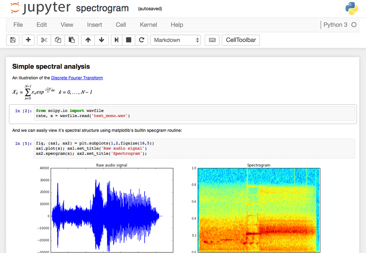
The Jupyter interface.
Where Did Jupyter Notebook Come From?
Project Jupyter evolved from the original IPython project to support multiple languages, leading to its name as the Jupyter Notebook. The name itself is a nod to its initial focus on JUlia, PYThon, and R (and is also inspired by the planet Jupiter).
When running Python in Jupyter, the IPython kernel powers your notebooks, giving you access to features that make coding smoother and more interactive (we’ll cover these soon!).
Now, let’s explore 28 practical tips to make your Jupyter experience smoother, faster, and more productive.
1. Jupyter Notebook Keyboard Shortcuts
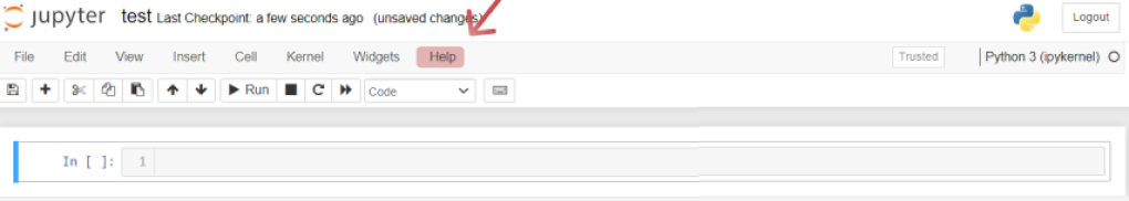
As any power user knows, keyboard shortcuts can save you significant time. Jupyter Notebook provides a built-in reference for these shortcuts under Help > Keyboard Shortcuts in the top menu. Alternatively, you can press H while in Command Mode to view the full list. It’s a good idea to check this list periodically, as new shortcuts may be added with updates.
Another helpful tool for navigating efficiently is the command palette, which can be accessed by pressing Cmd + Shift + P (or Ctrl + Shift + P on Windows and Linux). The command palette allows you to run any command by name, making it a useful alternative when you don’t remember a shortcut or if the action you want doesn’t have one. This functionality is similar to Spotlight search on a Mac, and once you get used to it, you’ll wonder how you worked without it!
The command palette provides an efficient way to run commands without needing to remember specific keyboard shortcuts.
Frequently Used Jupyter Notebook Keyboard Shortcuts:
Escswitches you to Command Mode, where you can navigate around your notebook using the arrow keys. You'll know you're in Command Mode when the notebook's cell border is blue, and no blinking text cursor is visible inside the cell.
<li>While in <b>Command Mode</b>:
    <ul>
        <li><code>A</code> inserts a new cell above the current cell, while <code>B</code> inserts one below.</li>
        <li><code>M</code> converts the current cell to a <b>Markdown</b> cell, and <code>Y</code> switches it back to a <b>Code</b> cell.</li>
        <li><code>D + D</code> (<i>press "D" twice</i>) deletes the selected cell.</li>
        <li><code>Z</code> undoes the deletion of a cell—perfect if you delete one by mistake.</li>
    </ul>
</li>

<li><code>Enter</code> switches you from <b>Command Mode</b> back to <b>Edit Mode</b>. In <b>Edit Mode</b>, the cell border turns green, and a blinking text cursor appears inside, allowing you to edit its content.</li>

<li>While in <b>Edit Mode</b>:
    <ul>
        <li><code>Shift + Enter</code> runs the cell and moves to the next one.</li>
        <li><code>Ctrl + Enter</code> runs the cell but keeps the focus on the same cell.</li>
        <li><code>Alt + Enter</code> runs the cell and inserts a new one below.</li>
        <li><code>Ctrl + ]</code> indents the selected lines, and <code>Ctrl + [</code> unindents them.</li>
        <li><code>Ctrl + /</code> toggles comments for selected lines of code.</li>
    </ul>
</li>

<li><code>Ctrl + Shift + -</code> splits the current cell into two at the cursor’s location.</li>
<li><code>Esc + F</code> opens the <b>Find and Replace</b> dialog, allowing you to search and replace within the code cells without affecting outputs.</li>
<li><code>Esc + O</code> toggles the output visibility of the current cell.</li>

<li>Selecting Multiple Cells:
    <ul>
        <li><code>Shift + J</code> (<i>or</i> <code>Shift + Down</code>) selects the next cell downward.
            <code>Shift + K</code> (<i>or</i> <code>Shift + Up</code>) selects the next cell upward.</li>
        <li>Once multiple cells are selected, you can delete, copy, cut, paste, or run them as a batch—making it easier to manage and reorganize your notebook.</li>
        <li><code>Shift + M</code> merges selected cells into one.</li>
    </ul>
</li>
Merging multiple cells.
2. Display Multiple Outputs in Jupyter Notebook Cells
By default, Jupyter Notebook only displays the output of the last command within a cell. For example, in the code below, only the output of quakes.tail(3) is shown:
from pydataset import data

quakes = data('quakes')
quakes.head(3)  # Output is not displayed
quakes.tail(3)  # Output is displayed
Output:
| lat | long | depth | mag | stations |
|---|---|---|---|---|
| -25.93 | 179.54 | 470 | 4.4 | 22 |
| -12.28 | 167.06 | 248 | 4.7 | 35 |
| -20.13 | 184.20 | 244 | 4.5 | 34 |
However, you can change this behavior to display all outputs by using the following Jupyter Notebook trick:
from IPython.core.interactiveshell import InteractiveShell
from pydataset import data

InteractiveShell.ast_node_interactivity = "all"

quakes = data('quakes')
quakes.head(3)  # Output is displayed
quakes.tail(3)  # Output is displayed
Output:
First 3 rows:
| lat | long | depth | mag | stations |
|---|---|---|---|---|
| -20.42 | 181.62 | 562 | 4.8 | 41 |
| -20.62 | 181.03 | 650 | 4.2 | 15 |
| -26.00 | 184.10 | 42 | 5.4 | 43 |
Last 3 rows:
| lat | long | depth | mag | stations |
|---|---|---|---|---|
| -25.93 | 179.54 | 470 | 4.4 | 22 |
| -12.28 | 167.06 | 248 | 4.7 | 35 |
| -20.13 | 184.20 | 244 | 4.5 | 34 |
If you want this behavior to persist across all your Jupyter environments (Notebook and Console), you can configure it by creating a file at ~/.ipython/profile_default/ipython_config.py with the following content:
c = get_config()
# Display all outputs in the cell
c.InteractiveShell.ast_node_interactivity = "all"
This configuration change can be especially useful when working with pandas DataFrames or when you need to compare multiple outputs in the same cell. It’s one of the many Jupyter Notebook tricks that can help you optimize your workflow and enhance productivity.
3. Easy Access to Documentation
Jupyter Notebook provides several ways to access documentation without leaving the interface, making it easy to get help when you need it. One option is through the Help menu, which includes links to online documentation for popular libraries like NumPy, pandas, SciPy, and Matplotlib.
Access library documentation through the Help menu.
Another useful method is using the built-in Docstring feature to view documentation for specific functions, methods, or variables. To do this, simply prepend the object with a question mark (?) and run the cell.
?str.replaceThe output will display the Docstring, explaining the syntax and functionality of the object:
Docstring:
S.replace(old, new[, count]) -> str

Return a copy of S with all occurrences of substring
old replaced by new. If the optional argument count is
given, only the first count occurrences are replaced.
Type:      method_descriptor
This feature is especially useful for quickly checking parameters and return types, saving you time as you work through your Jupyter Notebook.
4. Plotting in Notebooks
Jupyter Notebook supports several powerful libraries for creating both static and interactive visualizations directly within your notebook. Here’s a quick overview of popular options and when to use them:
- Matplotlib: The go-to plotting library in Python. Activate inline plots using
%matplotlib inline. For a guided introduction, check out this Matplotlib Tutorial.
<li><code>%matplotlib notebook</code>: Provides interactive plots with zooming and panning. However, rendering may be slower since it’s processed server-side.</li>
<li><a href="https://seaborn.pydata.org/" target="_blank" rel="noopener">Seaborn</a>: Built on top of Matplotlib, Seaborn simplifies creating elegant and informative visualizations. Just importing Seaborn will automatically enhance your Matplotlib plots.</li>
<li><a href="https://github.com/mpld3/mpld3" target="_blank" rel="noopener">mpld3</a>: Offers an alternative to Matplotlib using the d3.js library for interactive visualizations. Note that it has limited functionality compared to Matplotlib.</li>
<li><a href="https://bokeh.org/" target="_blank" rel="noopener">Bokeh</a>: Ideal for building interactive plots with dynamic features such as zooming, filtering, and live updates, making it a popular choice for creating dashboards.</li>
<li><a href="https://plotly.com/python/" target="_blank" rel="noopener">Plotly</a>: Known for producing high-quality interactive visualizations. Fully open source, Plotly supports hover tooltips, legends, and a variety of chart types.</li>
<li><a href="https://altair-viz.github.io/" target="_blank" rel="noopener">Altair</a>: A declarative visualization library that emphasizes simplicity and elegance. While easy to use, its customization options are more limited compared to Matplotlib.</li>
An example of an interactive Bokeh plot embedded within Jupyter.
5. IPython Magic Commands
Jupyter Notebook is built on the IPython kernel, giving you access to a wide range of powerful IPython Magic commands. These commands can enhance productivity and simplify your workflow, providing shortcuts for common tasks like plotting, system calls, and debugging.
To view all available magic commands, run the following in a cell:
%lsmagicThis will display a list of both line magics (which operate on a single line) and cell magics (which affect entire cells):
Available line magics:
%alias  %alias_magic  %autoawait  %autocall  %automagic  %autosave  %bookmark  %cat  %cd  %clear  %colors  %conda  %config  %connect_info  %cp  %debug  %dhist  %dirs  %doctest_mode  %ed  %edit  %env  %gui  %hist  %history  %killbgscripts  %ldir  %less  %lf  %lk  %ll  %load  %load_ext  %loadpy  %logoff  %logon  %logstart  %logstate  %logstop  %ls  %lsmagic  %lx  %macro  %magic  %man  %matplotlib  %mkdir  %more  %mv  %notebook  %page  %pastebin  %pdb  %pdef  %pdoc  %pfile  %pinfo  %pinfo2  %pip  %popd  %pprint  %precision  %prun  %psearch  %psource  %pushd  %pwd  %pycat  %pylab  %qtconsole  %quickref  %recall  %rehashx  %reload_ext  %rep  %rerun  %reset  %reset_selective  %rm  %rmdir  %run  %save  %sc  %set_env  %store  %sx  %system  %tb  %time  %timeit  %unalias  %unload_ext  %who  %who_ls  %whos  %xdel  %xmode

Available cell magics:
%%!  %%HTML  %%SVG  %%bash  %%capture  %%debug  %%file  %%html  %%javascript  %%js  %%latex  %%markdown  %%perl  %%prun  %%pypy  %%python  %%python2  %%python3  %%ruby  %%script  %%sh  %%svg  %%sx  %%system  %%time  %%timeit  %%writefile
Magic commands can be incredibly useful for tasks like debugging, profiling, or interacting with the system. If you’re new to magics, check out the official IPython Magic documentation for examples and explanations.
Stay tuned—we’ll highlight some of the most useful IPython magic commands in the upcoming sections to help you work more efficiently in your notebooks!
6. IPython Magic – %env: Set Environment Variables
When working with libraries like Theano or TensorFlow in Jupyter Notebook, you may need to adjust environment variables to control their behavior. Instead of restarting the Jupyter server every time you modify an environment variable, you can use the %env magic command to manage them directly within your notebook.
To list all current environment variables, simply run:
%envTo set an environment variable, use the following syntax:
%env VARIABLE_NAME=valueFor example, to set the OMP_NUM_THREADS environment variable to 4, you would run:
%env OMP_NUM_THREADS=4To confirm the value has been set, you can access it using Python’s os.environ:
import os
os.environ['OMP_NUM_THREADS']
This will output the value of the variable, verifying that it’s been set correctly:
'4'By using %env, you can quickly fine-tune your environment on the fly, making it especially useful when optimizing library performance or testing different configurations.
7. IPython Magic – %run: Reuse and Execute External Code
The %run magic command allows you to execute external Python files or entire Jupyter Notebooks directly within your current notebook. This is especially useful when you want to reuse code from previous projects without copying and pasting it into multiple notebooks.
To execute a Python script, provide the path to the file:
%run path/to/your/script.pyTo run another Jupyter Notebook, specify the path to the .ipynb file:
%run path/to/your/notebook.ipynbFor example, to execute a notebook named two_histograms.ipynb in the same directory as your current notebook, you would run:
%run ./two_histograms.ipynb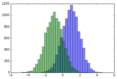
Keep in mind that %run executes the code in the current namespace, meaning variables and functions defined in the external file or notebook will be directly accessible in your current notebook. This is different from importing a module, where you typically need to use the module’s name as a prefix to access its functions and variables.
Using %run can help streamline your workflow and keep your projects organized by separating reusable code into external scripts or notebooks. This is one of the many useful Jupyter Notebook tips that can improve your productivity and reduce code duplication.
8. IPython Magic – %load: Insert Code from External Scripts
The %load magic command allows you to insert code from an external script directly into a cell of your Jupyter Notebook. This is useful when you want to quickly import and run code from a file without needing to copy and paste it manually.
To use %load, provide the path to the script you want to insert:
%load path/to/your/script.pyFor example, if you have a file named hello_world.py in the same directory as your notebook, you can load its code using:
%load ./hello_world.pyAfter running the cell, you’ll see that the contents of hello_world.py are automatically inserted into the cell, replacing the %load line:
if __name__ == "__main__":
    print("Hello World!")
When you execute the cell, you’ll get the following output:
Hello World!In addition to local files, you can also use %load with URLs to insert code from online sources, making it even more versatile when working with external resources.
This Jupyter Notebook tip highlights how the %load magic command can save time by quickly integrating external scripts into your notebook, helping you work more efficiently.
9. IPython Magic – %store: Pass Variables Between Notebooks
The %store magic command lets you pass variables between different notebooks, making it extremely useful for multi-notebook workflows and collaborative projects. Instead of manually copying values, you can easily share data across notebooks with just a few commands.
To store a variable for use in another notebook, use %store followed by the variable name:
data = 'this is the string I want to pass to a different notebook'
%store data
You’ll see confirmation that the variable has been stored:
Stored 'data' (str)After storing it, you can optionally remove the variable from the current notebook’s memory using:
del dataIn another notebook, retrieve the stored variable using %store -r followed by the variable name:
%store -r data
print(data)
The output will confirm the value of the retrieved variable:
this is the string I want to pass to a different notebookWith the %store magic command, you can effortlessly share variables between notebooks, simplifying workflows and enhancing collaboration on large projects.
10. IPython Magic – %who: List Variables in the Global Scope
The %who magic command allows you to list all variables currently in the global scope. This is especially useful when you’re working with many variables and need to see their names and types at a glance.
To display all variables in the global scope, run:
%whoThis will list all variables, regardless of their type.
If you only want to display variables of a specific type, you can pass the type as an argument to %who. For example, to see only string variables:
one = "for the money"
two = "for the show"
three = "to get ready now go cat go"

%who str
The output will list all string variables currently in the global scope:
one three twoThe %who magic command is a valuable Jupyter Notebook trick that helps you keep track of your variables, making it easier to maintain an organized and efficient coding environment.
11. IPython Magic – %timeit: Timing Code Execution
When your code is running slowly, timing its execution can help you identify bottlenecks and optimize performance. The %%time and %timeit magic commands are two powerful tools for this purpose.
%%time: Measure Execution Time for a Single Run
The %%time magic command measures the time taken to execute all the code in a cell and displays the CPU times and total elapsed time (wall time).
%%time
import time

for _ in range(1000):
    time.sleep(0.01)  # sleep for 0.01 seconds
The output will show detailed timing information:
CPU times: user 21.5 ms, sys: 14.8 ms, total: 36.3 ms
Wall time: 11.6 s%timeit: Measure Execution Time Across Multiple Runs
The %timeit magic command provides a more accurate performance measurement by executing the code multiple times (the default is 100,000 loops) and displaying the mean of the fastest runs.
import numpy as np

%timeit np.random.normal(size=100)
The output will include timing statistics:
9.29 µs ± 63.1 ns per loop (mean ± std. dev. of 7 runs, 100000 loops each)These Jupyter Notebook tips highlight how using %%time and %timeit can help you measure performance, pinpoint inefficiencies, and optimize your code for faster execution.
12. IPython Magic – %config: High-Resolution Plot Outputs for Retina Displays
When working on devices with high-resolution Retina displays, such as recent MacBook models, you might notice that plots generated in Jupyter Notebook look pixelated or blurry. Fortunately, with a simple IPython magic command, you can create double-resolution plots that take full advantage of your screen's capabilities.
Create a Sample Plot
Let’s start by generating a basic plot using Matplotlib:
import matplotlib.pyplot as plt

x = range(1000)
y = [i ** 2 for i in x]
plt.plot(x, y)
plt.show()
Enable High-Resolution Plotting
To display sharper plots on Retina displays, use the following magic command before your plotting code:
%config InlineBackend.figure_format = 'retina'

plt.plot(x, y)
plt.show()
Key Considerations
- Retina displays only: The high-resolution plot will only be visible on Retina displays. On standard displays, the plot will render at normal resolution.
- Better visualization: By setting
InlineBackend.figure_formatto'retina', Matplotlib generates plots with double the resolution, leading to sharper and more detailed visuals on supported devices.
This Jupyter Notebook tip demonstrates how a small configuration change can significantly improve the visual quality of your plots, making them look crisp and professional on high-resolution displays.
13. IPython Magic – %pdb: Debugging Your Code
The %pdb magic command lets you debug your code using the Python Debugger (pdb) directly within the Jupyter Notebook. This tip demonstrates how you can efficiently catch errors and inspect variables without leaving the notebook interface.
How to Use %pdb
Let’s say you have a function that calculates the average of a list of numbers but fails if the list is empty:
%pdb

def calculate_average(numbers):
    total = sum(numbers)
    count = len(numbers)
    return total / count  # This will raise ZeroDivisionError if the list is empty

# Call the function with an empty list to trigger the error
calculate_average([])
What Happens When an Exception Is Raised?
When the exception occurs, Jupyter automatically enters the pdb debugger. You’ll be able to examine the current state of the program, step through the code, and inspect variables to identify the issue.
Common pdb Commands
n(next): Execute the next line of code.s(step): Step into a function call.c(continue): Continue execution until the next breakpoint or exception.p var(print): Display the value of a variable namedvar.h(help): Display a list ofpdbcommands and their descriptions.q(quit): Exit the debugger.
Why Use %pdb?
Debugging directly in the notebook allows for an interactive and efficient workflow. By using %pdb, you can quickly identify and fix issues without needing to switch to an external debugger, saving time and effort when developing and testing your code.
14. Suppress the Output of a Final Function
Sometimes, when working in Jupyter Notebooks, you may notice that the output of a function appears alongside visualizations, like when using plotting libraries such as Matplotlib. This Jupyter Notebook trick allows you to suppress that extra output, keeping your notebook clean and focused.
Understanding the Issue
Let’s create a sample plot using Matplotlib:
%matplotlib inline
import matplotlib.pyplot as plt
import numpy as np

x = np.linspace(0, 1, 1000)**1.5
plt.hist(x)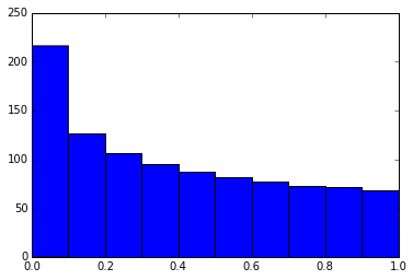
In addition to the histogram plot, the cell outputs extra information related to the plt.hist(x) function:
(array([216., 126., 106.,  95.,  87.,  81.,  77.,  73.,  71.,  68.]),
 array([0. , 0.1, 0.2, 0.3, 0.4, 0.5, 0.6, 0.7, 0.8, 0.9, 1. ]),
 <a list of 10 Patch objects>)
Solution: Suppress Output Using a Semicolon
To hide the extra output and display only the plot, add a semicolon (;) at the end of the function call:
plt.hist(x);
Why It Works
The semicolon suppresses the function’s return value from being displayed in the output cell, leaving only the plot visible. This simple Jupyter Notebook trick helps maintain a clean and professional notebook, especially when working with multiple plots or functions that produce verbose output.
15. Executing Shell Commands
Jupyter Notebook allows you to execute shell commands directly within cells, making it easier to manage files, install packages, and interact with the system without switching to an external terminal. This is done by prefixing the shell command with an exclamation mark (!).
Listing Files in the Directory
To list all CSV files in your current working directory, use the ls command with a wildcard (*) to match the file extension:
!ls *.csvThe output will display the list of matching files:
nba_2016.csv titanic.csv pixar_movies.csv whitehouse_employees.csvInstalling and Verifying Packages
You can install Python packages using the shell within the notebook and then verify the installation:
!pip install numpy
!pip list | grep pandas
The output will confirm the package installation and display the version:
Requirement already satisfied: numpy in /dataquest/system/env/python3/lib/python3.8/site-packages (1.24.4)
pandas              2.0.3
Why Use Shell Commands?
Shell commands in Jupyter streamline your workflow by letting you perform system-level tasks, manage files, and handle package installations all within the same notebook. This keeps your work centralized and allows for better project organization and reproducibility.
16. Using LaTeX for Formulas
One of my most favorite Jupyter Notebook tricks is the ability to embed beautifully rendered mathematical formulas using LaTeX within Markdown cells.
LaTeX is a typesetting language designed for creating well-structured documents, but it's particularly loved by mathematicians and scientists for its ability to render beautiful mathematical expressions. Instead of relying on plain text shortcuts to represent equations, LaTeX allows you to display mathematical symbols exactly as you’d remember them from math class—like the elegant summation \( \sum \) or integral \( \int \) symbols. This makes your equations not only more visually appealing but also easier for others to understand at a glance.
There are two main ways to use LaTeX:
- Inline Math Mode: Use single dollar signs (
$...$) to embed mathematical expressions directly within a line of text. - Display Math Mode: Use double dollar signs (
$$...$$) to center the expression and display it on its own line with larger formatting.
Literal LaTeX Input
Euler's identity (inline): $e^{i\pi} + 1 = 0$
Euler's identity (display):
$$
e^{i\pi} + 1 = 0
$$

Pythagorean theorem (inline): $a^2 + b^2 = c^2$
Pythagorean theorem (display):
$$
a^2 + b^2 = c^2
$$

Summation (inline): $\sum_{i=1}^{n} i = \frac{n(n+1)}{2}$
Summation (display):
$$
\sum_{i=1}^{n} i = \frac{n(n+1)}{2}
$$
Rendered Output
Euler's identity (inline): $e^{i\pi} + 1 = 0$
Euler's identity (display):
$$ e^{i\pi} + 1 = 0 $$
Pythagorean theorem (inline): $a^2 + b^2 = c^2$
Pythagorean theorem (display):
$$ a^2 + b^2 = c^2 $$
Summation (inline): $\sum_{i=1}^{n} i = \frac{n(n+1)}{2}$
Summation (display):
$$ \sum_{i=1}^{n} i = \frac{n(n+1)}{2} $$
By leveraging Markdown and LaTeX together, you can communicate complex mathematical concepts effectively. For more advanced equations and symbols, explore this LaTeX reference guide.
17. Run Code from Different Kernels in a Notebook
One of the most versatile Jupyter Notebook tricks I use is the ability to run code from multiple programming languages (or kernels) within a single notebook. This allows me to combine the strengths of different languages seamlessly, making my notebooks more powerful and efficient.
To use a specific kernel in a cell, prefix it with the corresponding IPython magic command:
%%bashfor Bash shell scripts%%HTMLfor HTML code%%python2for Python 2%%python3for Python 3%%rubyfor Ruby%%perlfor Perl
Example: Running Bash Commands
The %%bash magic command lets you execute Bash commands directly within a notebook cell. Here's an example that prints a sequence of numbers:
%%bash
for i in {1..5}
do
  echo "i is $i"
done
The output will display:
i is 1
i is 2
i is 3
i is 4
i is 5
Example: Running Ruby Code
You can also execute Ruby code using the %%ruby magic:
%%ruby
puts "Hello from Ruby!"
(1..5).each do |i|
  puts "Square of #{i} is #{i**2}"
end
The output will be:
Hello from Ruby!
Square of 1 is 1
Square of 2 is 4
Square of 3 is 9
Square of 4 is 16
Square of 5 is 25
This Jupyter Notebook magic command highlights the flexibility of the platform, allowing you to combine different languages in one environment. This can be particularly helpful when you need to perform tasks like shell scripting, web scraping, or data processing using specialized tools across multiple languages.
18. Install Other Kernels for Jupyter
One of Jupyter’s standout features is its ability to support multiple kernels, allowing you to run notebooks in different programming languages such as R, Julia, and more. This Jupyter Notebook tip walks you through the steps to install an R kernel using two methods.
Option 1: Installing the R Kernel Using Anaconda (Easiest Method)
If you set up your environment using Anaconda, installing the R kernel is straightforward. Simply run the following command in your terminal:
conda install -c r r-essentialsThe r-essentials package includes everything you need to start working with R in Jupyter, including the IRkernel and several popular R packages.
Option 2: Installing the R Kernel Manually
If you’re not using Anaconda, you’ll need to install R manually from CRAN. Once R is installed, open an R console and run the following commands:
install.packages(c('repr', 'IRdisplay', 'crayon', 'pbdZMQ', 'devtools'))
devtools::install_github('IRkernel/IRkernel')
IRkernel::installspec()  # Register the kernel in the current R installation
These commands will install the necessary dependencies and register the IRkernel with Jupyter, making it available as an option when creating new notebooks.
Using Other Kernels
In addition to R, Jupyter supports many other kernels, such as Julia, Scala, and more. For a complete list of supported kernels and installation instructions, check out the official Jupyter documentation.
By installing additional kernels, you can make Jupyter a truly multi-language environment, allowing you to work seamlessly across different programming languages within the same interface.
19. IPython Magic – %load_ext: Enable and Manage Extensions
The %load_ext magic command lets you enable extensions that provide additional functionalities within Jupyter notebooks. These extensions can be useful for debugging, formatting, or profiling your code, among other tasks.
To load an extension, simply specify its name:
%load_ext extension_nameFor example, to load the autoreload extension, which automatically reloads modules before executing cells, run:
%load_ext autoreloadYou can then configure the extension. For example, to automatically reload all modules before each execution:
%autoreload 2If you no longer need the extension during the session, you can disable it using:
%unload_ext extension_nameThe %load_ext magic command simplifies enabling extensions, enhancing your workflow and allowing you to customize Jupyter notebooks with additional tools tailored to your needs.
20. Writing Functions in Other Languages
Sometimes, the speed of numpy just isn’t good enough for certain tasks, and I need to implement faster code. Sure, you could compile functions into dynamic libraries and manually write Python wrappers… but isn’t it much better when this boring part is done for you?
Fortunately, Jupyter makes it easy to write functions in Cython or Fortran and use them directly in your Python code. Here’s how to get started:
Writing Functions with Cython
First, install the necessary packages:
!pip install cython fortran-magicNext, load the Cython extension into your notebook:
%load_ext CythonYou can now write Cython functions using the %%cython cell magic:
%%cython

def multiply_by_2(float x):
    return 2.0 * x
To test the function, pass a value and see the result:
multiply_by_2(23.0)Writing Functions with Fortran
Personally, I prefer using Fortran when writing number-crunching functions. I’ve found it to be really convenient, especially for scientific computing tasks. To get started, load the Fortran magic extension:
%load_ext fortranmagicYou can now write Fortran subroutines directly in your notebook using the %%fortran cell magic:
%%fortran
subroutine compute_fortran(x, y, z)
    real, intent(in) :: x(:), y(:)
    real, intent(out) :: z(size(x, 1))
    z = sin(x + y)
end subroutine compute_fortran
To test the subroutine, pass arrays and view the output:
compute_fortran([1, 2, 3], [4, 5, 6])Additional Resources and Tips
If you’d like to dive deeper into using Fortran with Python, I highly recommend checking out this detailed guide. It walks you through how to get the most out of Fortran when writing high-performance code.
There are also different just-in-time (JIT) compilation tools that can speed up your Python code. For example, this speed benchmark guide compares various methods and can help you decide which one works best for your needs.
With tools like Cython and Fortran, you can optimize your code for high performance without the headache of writing complex wrappers. I’ve personally found these techniques to be lifesavers when working on projects involving large datasets and intensive computations.
21. Multicursor Support
Jupyter Notebooks support multiple cursors, a feature similar to what you’d find in code editors like Sublime Text or VS Code. This can be a game-changer when editing repetitive code or making bulk changes within cells.
To enable multicursor mode, simply click and drag your mouse while holding down Alt (or Option on macOS).
Multicursor support in action.
Alternatively, you can hold down Ctrl (or Cmd on macOS) and click at multiple locations within the cell to create cursors exactly where you need them. This method gives you precise control, which is especially useful when working with large blocks of code.
22. Jupyter-contrib Extensions
Jupyter-contrib extensions are a collection of community-driven enhancements that add extra functionality to Jupyter Notebooks. Some popular extensions include a spell-checker, code formatter, table of contents generator, and more. These extensions can significantly boost productivity and streamline your notebook workflow.
Installing Jupyter-contrib Extensions
To install these extensions and the configurator menu, which lets you browse and enable them from the Jupyter interface, run the following commands:
!pip install https://github.com/ipython-contrib/jupyter_contrib_nbextensions/tarball/master
!pip install jupyter_nbextensions_configurator
!jupyter contrib nbextension install --user
!jupyter nbextensions_configurator enable --user
Once installed, you can access the nbextensions tab from the Jupyter Notebook home screen. From there, you can browse available extensions and enable them with a single click.
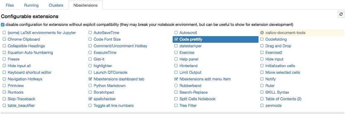
The nbextensions configurator interface.
23. Create a Presentation from a Jupyter Notebook
Have you ever wanted to present your Jupyter Notebook as an interactive slideshow without exporting it to another tool? With the RISE extension, you can do just that—directly within the notebook interface.
Installing RISE
You can install RISE using either conda or pip, depending on your preferred package manager:
Using Conda:
conda install -c conda-forge riseUsing Pip:
pip install riseEnabling the Extension
Once installed, enable RISE with the following commands:
jupyter-nbextension install rise --py --sys-prefix
jupyter-nbextension enable rise --py --sys-prefix
Starting Your Presentation
After enabling RISE, open your notebook and click the "Enter/Exit RISE Slideshow" button in the toolbar. You can navigate the slides using the arrow keys.
Customizing Slide Types
RISE allows you to control the flow of your presentation by specifying different slide types. Here are some helpful shortcuts for setting slide types:
Shift + M: Regular slide (Markdown cell)Shift + J: Regular slide (Code cell)Shift + F: Fragment slide (Markdown cell)Shift + H: Sub-slide (Markdown cell)Shift + N: Skip slide (Markdown cell)
With RISE, you can turn your data exploration and analysis into engaging presentations directly from your Jupyter Notebook, making it easy to share insights interactively.
24. The Jupyter Output System
Jupyter Notebooks are displayed as HTML, and their cell outputs can also be HTML. This means you can return almost any type of media, including text, images, audio, and video, directly in your notebook cells.
Displaying Images from a Folder
In this example, we scan a folder containing images and display thumbnails of the first five:
import os
from IPython.display import display, Image

# List PNG files in the specified directory
names = [f for f in os.listdir('../images/ml_demonstrations/') if f.endswith('.png')]

# Display the first five images as thumbnails
for name in names[:5]:
    display(Image('../images/ml_demonstrations/' + name, width=100))
The output displays thumbnails of the images:


Generating the Same List Using Shell Commands
You can achieve the same result using a Bash command within a notebook cell. Jupyter magic commands allow shell outputs to be captured as Python variables:
# Get a list of PNG files using a shell command
names = !ls ../images/ml_demonstrations/*.png

# Display the first five filenames
names[:5]
[
'../images/ml_demonstrations/colah_embeddings.png',
'../images/ml_demonstrations/convnetjs.png',
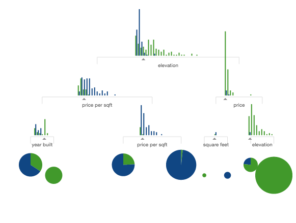
'../images/ml_demonstrations/decision_tree.png',
'../images/ml_demonstrations/decision_tree_in_course.png',
'../images/ml_demonstrations/dream_mnist.png'
]The Jupyter output system’s flexibility allows you to explore, visualize, and manage data seamlessly by combining Python and shell commands in one environment.
25. Enhance Interactivity with ipywidgets
ipywidgets is a powerful library that brings interactivity to your Jupyter notebooks. With widgets like sliders, buttons, checkboxes, and dropdowns, you can manipulate data in real-time, making your notebooks more dynamic and engaging.
Installation
To get started, make sure ipywidgets is installed:
!pip install ipywidgetsCreating and Displaying Widgets
Import ipywidgets and the display function from IPython.display:
import ipywidgets as widgets
from IPython.display import display
Let’s create a simple slider widget:
slider = widgets.FloatSlider(
    value=5.0,
    min=0.0,
    max=10.0,
    step=0.1,
    description='Value:'
)
display(slider)
This slider has a default value of 5.0, a range from 0.0 to 10.0, and a step size of 0.1. The description parameter adds a label to the slider.
Accessing Widget Values
To access the current value of the slider, use its value attribute:
print(slider.value)Interactive Button Example
ipywidgets also lets you create interactive buttons that trigger events. Let’s build a button that prints a message when clicked:
button = widgets.Button(description='Click me!')
output = widgets.Output()

def on_button_clicked(b):
    with output:
        print("Hello, Jupyter!")

button.on_click(on_button_clicked)
display(button, output)
When you click the button, the message "Hello, Jupyter!" will be printed inside the output widget.
Explore More Widgets
In addition to sliders and buttons, ipywidgets offers many other widgets like checkboxes, dropdowns, and text boxes. By using these widgets, you can transform your notebooks into interactive dashboards or teaching tools, enhancing the learning and exploratory experience.
26. Big Data Analysis
Jupyter Notebooks offer several options for querying and processing large datasets, making it easier to work with big data directly from within your notebook environment. Here are some popular solutions:
- Dask: A powerful library for parallel and distributed computing in Python, Dask scales your computations from a single machine to a large cluster without needing to change much code. It integrates seamlessly with pandas, NumPy, and other libraries.
- Ray: Designed for scalable, distributed applications, Ray is ideal for parallel model training, hyperparameter tuning, and general distributed workloads.
- PySpark: Integrates the power of Apache Spark with the simplicity of Python, enabling distributed data processing and analysis on large datasets.
-
spark-sql magic: This enables SQL queries directly within your notebook using
%%sql, providing an interactive way to query large datasets. Alternatively, you can explore newer options like Dask SQL or Databricks notebooks.
With these options, Jupyter Notebooks give you the flexibility to process and analyze large-scale data efficiently, making them a valuable tool for big data projects in data science and engineering.
27. Set an Alarm for Code Completion
Adding just a few lines of code can enable Python to play a sound or even speak to you when your code execution is complete. This provides a convenient way to stay informed about long-running tasks without constantly monitoring the notebook.
For Windows Users:
Use the built-in winsound module to create a simple beep:
import winsound

duration = 1000  # milliseconds
freq = 440  # Hz
winsound.Beep(freq, duration)
This code snippet will play a beep sound at a frequency of 440 Hz for 1 second when your code has finished running.
For Mac Users:
Use the built-in say command:
import os

os.system('say "Your program has finished"')
This will make your Mac speak the phrase "Your program has finished" once the code execution is complete. You can customize the voice using:
os.system('say -v Alex "Your program has finished"')For Linux Users:
First, install the sox package if it’s not already installed:
sudo apt-get install soxThen, use this command to play a beep sound:
import os

os.system('play -nq -t alsa synth 1 sine 440')
Cross-Platform Option:
To ensure compatibility across Windows, Mac, and Linux, you can use the playsound library to play audio files. First, install it using:
pip install playsoundThen, use the following code to play a sound file of your choice:
from playsound import playsound

playsound('path/to/sound.mp3')
This flexible approach lets you play custom audio notifications regardless of your operating system.
By adding simple audio notifications, you can stay informed about long-running tasks without needing to constantly check your Jupyter Notebook.
28. Sharing Jupyter Notebooks
The easiest way to share your notebook is by sharing the notebook file (.ipynb) directly. However, if the recipient doesn’t have Jupyter installed, you can use one of these options:
- Convert to HTML: Use the
File > Download as > HTMLoption to convert and share an HTML version of your notebook, which can be viewed in any browser.
<li><strong>Upload to Google Colab:</strong> Upload your <code>.ipynb</code> file to <a href="https://colab.research.google.com/notebooks/intro.ipynb" target="_blank" rel="noopener">Google Colab</a>, a free online environment for running notebooks without local installation.</li>
<li><strong>Share via GitHub or Gists:</strong> Upload your notebook to <a href="https://gist.github.com/" target="_blank" rel="noopener">Gists</a> or GitHub, which both natively render notebooks. See <a href="https://github.com/dataquestio/solutions/blob/master/Lesson202Solution.ipynb" target="_blank" rel="noopener">this example</a> as a reference.
<ul>
<li><strong>Bonus:</strong> Use <a href="https://mybinder.org/" target="_blank" rel="noopener">mybinder</a> to provide up to 30 minutes of interactive Jupyter access directly from a GitHub repository.</li>
</ul>
</li>
<li><strong>Set up a multi-user environment with JupyterHub:</strong> For workshops or courses, consider <a href="https://github.com/jupyterhub/jupyterhub" target="_blank" rel="noopener">JupyterHub</a>. This setup allows multiple users to access notebooks without needing local installations.</li>
<li><strong>Host with Dropbox and render with nbviewer:</strong> Store your notebook on Dropbox or a similar file-sharing service and generate a shareable link. Then, use <a href="https://nbviewer.jupyter.org/" target="_blank" rel="noopener">nbviewer</a> to render and view the notebook directly from the link.</li>
<li><strong>Export as PDF:</strong> Use <code>File > Download as > PDF</code> to create a PDF version. For tips on creating polished, publication-ready notebooks, check out <a href="https://blog.juliusschulz.de/blog/ultimate-ipython-notebook" target="_blank" rel="noopener">Julius Schulz’s guide</a>.</li>
<li><strong>Create a blog post using Pelican:</strong> Convert notebooks into blog posts with <a href="/blog/how-to-setup-a-data-science-blog/" target="_blank" rel="noopener">Pelican</a>, a static site generator for Python-based blogs.</li>Tip: Choose your sharing method based on your audience—HTML files and Google Colab links are great for non-technical users, while GitHub repositories and JupyterHub setups are ideal for technical collaborators.
Next Steps
At Dataquest, our interactive guided projects use Jupyter notebooks and JupyterLab, so you can work on real data science projects while building job-ready skills. If you’re interested, you can sign up and complete our first module for free.
I hope you've enjoyed my favorite Jupyter Notebook tips and tricks. If you want to go even deeper, here are some additional resources I recommend to further enhance your understanding of Jupyter Notebook:
- IPython Magic Commands Documentation – Learn how to use powerful magic commands to streamline your workflow.
- ipywidgets Documentation – Build interactive widgets to enhance notebook interactivity.
- Profiling and Timing Python Code – Learn how to time and optimize your Python code effectively.
- MyBinder – Share and run Jupyter notebooks online without local setup.
- 4 Ways to Extend Jupyter Notebooks – Learn how to customize and extend notebooks to meet advanced needs.