How to Implement a B-Tree Data Structure
Rudolf Bayer and Edward M. McCreight coined the term B-tree data structure at the Boeing Research Labs in 1971. They published a scientific paper titled "Organization and maintenance of large ordered indices" and introduced a new data structure for fast data retrieval from disks. Although the B-tree data structure has evolved over the decades, understanding its concepts is still valuable.
Here's what we'll cover in this tutorial:
- B-tree data structures
- B-tree properties
- Traversing in a B-tree
- Searching in a B-tree
- Inserting a key in a B-tree
- Deleting a key in a B-tree
Let's get started!
What Is a B-Tree Data Structure?
A B-tree is a self-balanced tree data structure that is a generalized form of the Binary Search Tree (BST). However, unlike a binary tree, each node can have more than two children. In other words, each node can have up to m children and m-1 keys; also, each node must have at least $\lceil \frac{m}{2} \rceil$ children to keep the tree balanced. These features keep the tree’s height relatively small.
A B-tree data structure keeps the data sorted and allows searching, inserting, and deleting operations performed in amortized logarithmic time. To be more specific, the time complexity for accomplishing the mentioned operations is $O(log {n})$, where n is the number of keys stored in the tree.
Let’s assume we have to store a tremendous amount of data in a computer system. In this common situation, we're definitely unable to store the whole data in the main memory (RAM), and most of the data should be kept on disks. We also know that the secondary storage (various types of disks) is much slower than RAM. So, when we have to retrieve the data from the secondary storage, we need optimized algorithms to reduce the number of disk access.
The B-Tree data structure tries to minimize the number of disk access using advanced techniques and optimized algorithms for searching, inserting, and deleting, all of which allow the B-tree to stay balanced and, therefore, ensure finding data in logarithmic time.
To reveal how powerful B-tree is in minimizing disk access, let’s refer to the book Introduction to Algorithms, which proves that a B-tree with a height of two and 1001 children is able to store more than one billion keys. Still, only a disk access of two is required to find any key (Cormen et al., 2009).
We'll discuss the properties of B-tree and how it works in the following sections.
B-Tree Properties
There are three types of nodes in a B-tree of order m, and each of them has the following properties:
- Root Node
- A root node has between $2$ and $m$ children.
- Internal Nodes
- Each internal node has between $\lceil \frac{m}{2} \rceil$ and $m$ children — both ends are included.
- Each internal node may contain up to $m-1$ keys.
- Leaf Nodes
- All leaf nodes are at the same level.
- Each leaf node stores between $\lceil \frac{m-1}{2} \rceil$ and $m-1$ keys — both ends are included.
-
The height of a B-Tree can be yielded via the following equation:
$h \leq log _{m}{\frac{n+1}{2}}$, where m is the minimum degree and n is the number of keys.
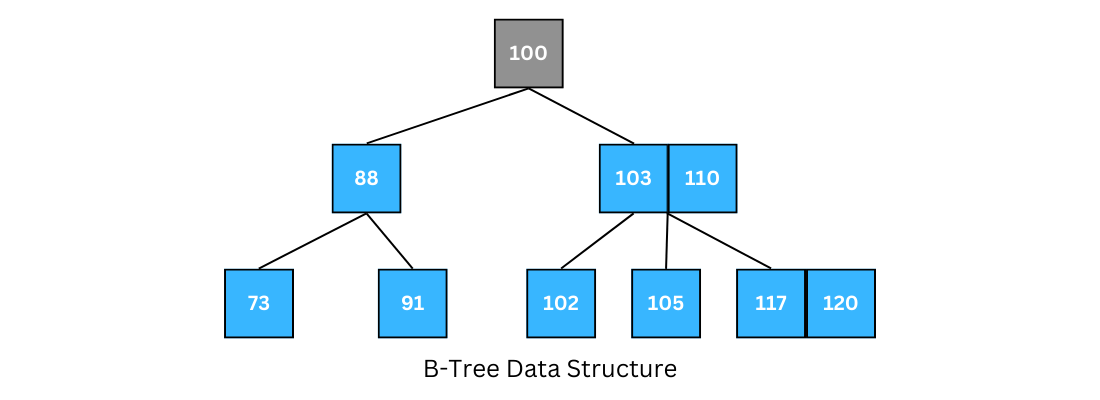
The illustration below shows a B-tree data structure.
Traversing in a B-Tree
To traverse a B-Tree, the traversal program starts from the leftmost child and prints its keys recursively. It repeats the same process for the remaining children and keys until the rightmost child.
Searching in a B-Tree
Searching for a specific key in a B-Tree is a generalized form of searching in a Binary Search Tree (BST). The only difference is that the BST performs a binary decision, but in the B-tree, the number of decisions at each node is equal to the number of the node's children.
Let's search key 102 in the B-tree above:
- The root's key is not equal to 102, so since k > 100, go to the leftmost node of the right branch.
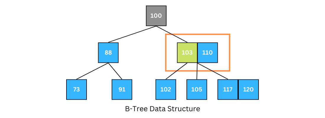
-
Compare k with 103; since k < 103, go to the left branch of the current node.
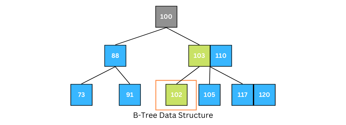
-
Compare k with the leaf's key; k exists there.
As shown, if the key we're looking for isn't in the range of the parent node, then most likely the key is in another branch. The algorithm will keep doing this to reach a leaf node. If it doesn't find the key, the algorithm returns NULL.
Inserting a Key in a B-Tree
So far, we've discussed traversing a B-tree and searching for a specific key in a B-tree data structure. This section will discuss how we can insert a new key into a B-Tree.
Inserting a new node into a B-tree includes two steps: finding the correct node to insert the key and splitting the node if the node is full (the number of the node’s keys is greater than m-1).
- If the B-Tree is empty:
- Allocate a root node, and insert the key.
- If the B-Tree is not empty:
- Find the proper node for insertion.
- If the node is not full:
- Insert the key in ascending order.
- If the node is full:
- Split the node at the median.
- Push the median key upward, and make the left keys a left child node and the right keys a right child node.
Deleting a Key in a B-Tree
Deletion is one of the operations we can perform on a B-tree. We can perform the deletion at the leaf or internal node levels. To delete a node from a B-tree, we need to follow the algorithm below:
-
If the node to delete is a leaf node:
- Locate the leaf node containing the desired key.
- If the node has at least $\lfloor \frac{m}{2} \rfloor$ keys, delete the key from the leaf node.
- If the node has less than $\lfloor \frac{m}{2} \rfloor$ keys, take a key from its right or left immediate sibling nodes. To do so, do the following:
- If the left sibling has at least $\lfloor \frac{m}{2} \rfloor$ keys, push up the in-order predecessor, the largest key on the left child, to its parent, and move a proper key from the parent node down to the node containing the key; then, we can delete the key from the node.
- If the right sibling has at least $\lfloor \frac{m}{2} \rfloor$ keys, push up the in-order successor, the smallest key on the right child, to its parent and move a proper key from the parent node down to the node containing the key; then, we can delete the key from the node.
- If the immediate siblings don't contain at least $\lfloor \frac{m}{2} \rfloor$ keys, create a new leaf node by joining two leaf nodes and the parent node's key.
- If the parent is left with less than $\lfloor \frac{m}{2} \rfloor$ keys, apply the above process to the parent until the tree becomes a valid B-Tree.
-
If the node to delete is an internal node:
- Replace it with its in-order successor or predecessor. Since the successor or predecessor will always be on the leaf node, the process will be similar as the node is being deleted from the leaf node.
Conclusion
This tutorial discussed B-trees and the application of B-trees for storing a large amount of data on disks. We also discussed four primary operations in B-trees: traversing, searching, inserting, and deleting. If you're interested in learning more about the actual implementation of a B-tree in Python, this GitHub repo shares the implementation of the B-tree data structure in Python.
I hope that you have learned something new today. Feel free to connect with me on LinkedIn or Twitter.