SQL Basics — Hands-On Beginner SQL Walkthrough Analyzing Bike-Sharing

In this beginner SQL walkthrough, we'll be working with a dataset from the bike-sharing service Hubway, which includes data on over 1.5 million trips made with the service.

We'll start by looking a little bit at databases, what they are and why we use them, before starting to write some queries of our own in SQL.

If you'd like to follow along you can download the hubway.db file here (130 MB).

SQL Basics: Relational Databases

A relational database is a database that stores related information across multiple tables and allows you to query information in more than one table at the same time.

It's easier to understand how this works by thinking through an example. Imagine you're a business and you want to keep track of your sales information. You could set up a spreadsheet in Excel with all of the information you want to keep track of as separate columns: Order number, date, amount due, shipment tracking number, customer name, customer address, and customer phone number.

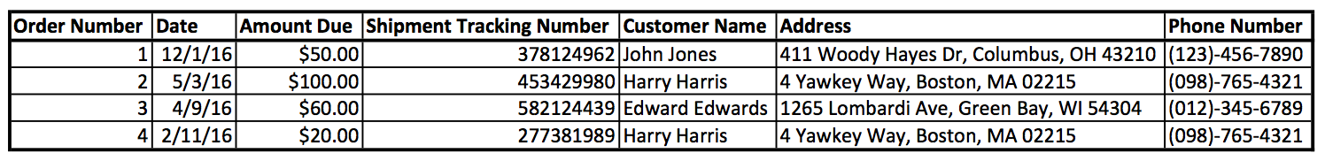
This setup would work fine for tracking the information you need to begin with, but as you start to get repeat orders from the same customer you'll find that their name, address and phone number gets stored in multiple rows of your spreadsheet.

As your business grows and the number of orders you're tracking increases, this redundant data will take up unnecessary space and generally decrease the efficiency of your sales tracking system. You might also run into issues with data integrity. There's no guarantee, for example, that every field will be populated with the correct data type or that the name and address will be entered exactly the same way every time.

With a relational database, like the one in the above diagram, you avoid all of these issues. You could set up two tables, one for orders and one for customers. The 'customers' table would include a unique ID number for each customer, along with the name, address and phone number we were already tracking. The 'orders' table would include your order number, date, amount due, tracking number and, instead of a separate field for each item of customer data, it would have a column for the customer ID.

This enables us to pull up all of the customer info for any given order, but we only have to store it once in our database rather than listing it out again for every single order.

Our Data Set

Let's start by taking a look at our database. The database has two tables, trips and stations. To begin with, we'll just look at the trips table. It contains the following columns:

• id — A unique integer that serves as a reference for each trip
• duration — The duration of the trip, measured in seconds
• start_date — The date and time the trip began
• start_station — An integer that corresponds to the id column in the stations table for the station the trip started at
• end_date — The date and time the trip ended
• end_station — The 'id' of the station the trip ended at
• bike_number — Hubway's unique identifier for the bike used on the trip
• sub_type — The subscription type of the user. "Registered" for users with a membership, "Casual" for users without a membership
• zip_code — The zip code of the user (only available for registered members)
• birth_date — The birth year of the user (only available for registered members)
• gender — The gender of the user (only available for registered members)

Our Analysis

With this information and the SQL commands we'll learn shortly, here are some questions that we'll try to answer over the course of this post:

• What was the duration of the longest trip?
• How many trips were taken by 'registered' users?
• What was the average trip duration?
• Do registered or casual users take longer trips?
• Which bike was used for the most trips?
• What is the average duration of trips by users over the age of 30?

The SQL commands we'll use to answer these questions are:

• SELECT
• WHERE
• LIMIT
• ORDER BY
• GROUP BY
• AND
• OR
• MIN
• MAX
• AVG
• SUM
• COUNT

Installation and Setup

For the purposes of this walkthrough, we will be using a database system called SQLite3. SQLite has come as part of Python from version 2.5 onwards, so if you have Python installed you'll almost certainly have SQLite as well. Python and the SQLite3 library can easily be installed and set up with Anaconda if you don't already have them.

Using Python to run our SQL code allows us to import the results into a Pandas dataframe to make it easier to display our results in an easy to read format. It also means we can perform further analysis and visualization on the data we pull from the database, although that will be beyond the scope of this post.

Alternatively, if we don't want to use or install Python, we can run SQLite3 from the command line. Simply download the "precompiled binaries" from the SQLite3 web page and use the following code to open the database:

~$ sqlite hubway.db SQLite version 3.14.0 2016-07-26 15:17:14Enter ".help" for usage hints.sqlite>

From here we can just type in the query we want to run and we will see the data returned in our terminal window.

An alternative to using the terminal is to connect to the SQLite database via Python. This would allow us to use a Jupyter notebook, so that we could see the results of our queries in a neatly formatted table.

To do this, we'll define a function that takes our query (stored as a string) as an input and shows the result as a formatted dataframe:

import sqlite3
span class="token keyword">import pandas as pd
b = sqlite3.connect('hubway.db')
span class="token keyword">def run_query(query):
   return pd.read_sql_query(query,db)

Of course, we don't have to use Python with SQL. If you're an R programmer already, our SQL Fundamentals for R Users course would be a great place to start.

SELECT

The first command we'll work with is SELECT. SELECT will be the foundation of almost every query we write - it tells the database which columns we want to see. We can either specify columns by name (separated by commas) or use the wildcard * to return every column in the table.

In addition to the columns we want to retrieve, we also have to tell the database which table to get them from. To do this we use the keyword FROM followed by the name of the table. For example, if we wanted to see the start_date and bike_number for every trip in the trips table, we could use the following query:

SELECT start_date, bike_number FROM trips;

In this example, we started with the SELECT command so that the database knows we want it to find us some data. Then we told the database we were interested in the start_date and bike_number columns. Finally we used FROM to let the database know that the columns we want to see are part of the trips table.

One important thing to be aware of when writing SQL queries is that we'll want to end every query with a semicolon (;). Not every SQL database actually requires this, but some do, so it's best to form this habit.

LIMIT

The next command we need to know before we start to run queries on our Hubway database is LIMIT. LIMIT simply tells the database how many rows you want it to return.

The SELECT query we looked at in the previous section would return the requested information for every row in the trips table, but sometimes that could mean a lot of data. We might not want all of it. If, instead, we wanted to see the start_date and bike_number for the first five trips in the database, we could add LIMIT to our query as follows:

SELECT start_date, bike_number FROM trips LIMIT 5;

We simply added the LIMIT command and then a number representing the number of rows we want to be returned. In this instance we used 5, but you can replace that with any number to get the appropriate amount of data for the project you're working on.

We will use LIMIT a lot in our queries on the Hubway database in this post — the trips table contains over a 1.5 million rows of data and we certainly don't need to display all of them!

Let's run our first query on the Hubway database. First we will store our query as a string and then use the function we defined earlier to run it on the database. Take a look at the following example:

query = 'SELECT * FROM trips LIMIT 5;'
un_query(query)

This query uses * as a wildcard instead of specifying columns to return. This means the SELECT command has given us every column in the trips table. We also used the LIMIT function to restrict the output to the first five rows of the table.

You will often see that people capitalize the commmand keywords in their queries (a convention that we'll follow throughout this post) but this is mostly a matter of preference. This capitalization makes the code easier to read, but it doesn't actually affect the code's function in any way. If you prefer to write your queries with lowercase commands, the queries will still execute correctly.

Our previous example returned every column in the trips table. If we were only interested in the duration and start_date columns, we could replace the wildcard with the column names as follows:

query = 'SELECT duration, start_date FROM trips LIMIT 5'
un_query(query)

ORDER BY

The final command we need to know before we can answer the first of our questions is ORDER BY. This command allows us to sort the database on a given column.

To use it, we simply specify the name of the column we would like to sort on. By default, ORDER BY sorts in ascending order. If we would like to specify which order the database should be sorted, we can add the keyword ASC for ascending order or DESC for descending order.

For example, if we wanted to sort the trips table from the shortest duration to the longest we could add the following line to our query:

ORDER BY duration ASC

With the SELECT, LIMIT and ORDER BY commands in our repertoire, we can now attempt to answer our first question: What was the duration of the longest trip?

To answer this question, it's helpful to break it down into sections and identify which commands we will need to address each part.

First we need to pull the information from the duration column of the trips table. Then, to find which trip is the longest, we can sort the duration column in descending order. Here's how we might work this through to come up with a query that will get the information we're looking for:

• Use SELECT to retrieve the duration column FROM the trips table
• Use ORDER BY to sort the duration column and use the DESC keyword to specify that you want to sort in descending order
• Use LIMIT to restrict the output to 1 row

Using these commands in this way will return the single row with the longest duration, which will provide us the answer to our question.

One more thing to note — as your queries add more commands and get more complicated, you may find it easier to read if you separate them onto multiple lines. This, like capitalization, is a matter of personal preference. It doesn't affect how the code runs (the system just reads the code from the beginning until it reaches the semicolon), but it can make your queries clearer and easier to follow. In Python, we can separate a string onto multiple lines by using triple quote marks.

Let's go ahead and run this query and find out how long the longest trip lasted.

query = '''
ELECT duration FROM trips
RDER BY duration DESC
IMIT 1;
''
un_query(query)

Now we know that the longest trip lasted 9999 seconds, or a little over 166 minutes. With a maximum value of 9999, however, we don't know whether this is really the length of the longest trip or if the database was only set up to allow a four digit number.

If it's true that particularly long trips are being cut short by the database, then we might expect to see a lot of trips at 9999 seconds where they reach the limit. Let's try running the same query as before, but adjust the LIMIT to return the 10 highest durations to see if that's the case:

query = '''
ELECT durationFROM trips
RDER BY duration DESC
IMIT 10
''
un_query(query)

What we see here is that there aren't a whole bunch of trips at 9999, so it doesn't look like we're cutting off the top end of our durations, but it's still difficult to tell whether that's the real length of the trip or just the maximum allowed value.

Hubway charges additional fees for rides over 30 minutes (somebody keeping a bike for 9999 seconds would have to pay an extra $25 in fees) so it's plausible that they decided 4 digits would be sufficient to track the majority of rides.

WHERE

The previous commands are great for pulling out sorted information for particular columns, but what if there is a specific subset of the data we want to look at? That's where WHERE comes in. The WHERE command allows us to use a logical operator to specify which rows should be returned. For example you could use the following command to return every trip taken with bike B00400:

WHERE bike_number = "B00400"

You'll also notice that we use quote marks in this query. That's because the bike_number is stored as a string. If the column contained numeric data types the quote marks would not be necessary.

Let's write a query that uses WHERE to return every column in the trips table for each row with a duration longer than 9990 seconds:

query = '''
ELECT * FROM trips
HERE duration > 9990;
''
un_query(query)

As we can see, this query returned 14 different trips, each with a duration of 9990 seconds or more. Something that stands out about this query is that all but one of the results has a sub_type of "Casual". Perhaps this is an indication that "Registered" users are more aware of the extra fees for long trips. Maybe Hubway could do a better job of conveying their pricing structure to Casual users to help them avoid overage charges.

We can already see how even a beginner-level command of SQL can help us answer business questions and find insights in our data.

Returning to WHERE, we can also combine multiple logical tests in our WHERE clause using AND or OR. If, for example, in our previous query we had only wanted to return the trips with a duration over 9990 seconds that also had a sub_type of Registered, we could use AND to specify both conditions.

Here's another personal preference recommendation: use parentheses to separate each logical test, as demonstrated in the code block below. This isn't strictly required for the code to function, but parentheses make your queries easier to understand as you increase the complexity.

Let's run that query now. We already know it should only return one result, so it should be easy to check that we've got it right:

query = '''
ELECT * FROM trips
HERE (duration >= 9990) AND (sub_type = "Registered")
RDER BY duration DESC;
''
un_query(query)

The next question we set out at the beginning of the post is "How many trips were taken by 'registered' users?" To answer it, we could run the same query as above and modify the WHERE expression to return all of the rows where sub_type is equal to 'Registered' and then count them up.

However, SQL actually has a built-in command to do that counting for us, COUNT.

COUNT allows us to shift the calculation to the database and save us the trouble of writing additional scripts to count up results. To use it, we simply include COUNT(column_name) instead of (or in addition to) the columns you want to SELECT, like this:

SELECT COUNT(id)
span class="token keyword">FROM trips

In this instance, it doesn't matter which column we choose to count because every column should have data for each row in our query. But sometimes a query might have missing (or "null") values for some rows. If we're not sure whether a column contains null values we can run our COUNT on the id column — the id column is never null, so we can be sure our count won't have missed anything.

We can also use COUNT(1) or COUNT(*) to count up every row in our query. It's worth noting that sometimes we might actually want to run COUNT on a column with null values. For example, we might want to know how many rows in our database have missing values for a column.

Let's take a look at a query to answer our question. We can use SELECT COUNT(*) to count up the total number of rows returned and WHERE sub_type = "Registered" to make sure we only count up the trips taken by Registered users.

query = '''
ELECT COUNT(*)FROM trips
HERE sub_type = "Registered";
''
un_query(query)

This query worked, and has returned the answer to our question. But the column heading isn't particularly descriptive. If someone else were to look at this table, they wouldn't be able to understand what it meant.
If we want to make our results more readable, we can use AS to give our output an alias (or nickname). Let's re-run the previous query but give our column heading an alias of Total Trips by Registered Users:

query = '''
ELECT COUNT(*) AS "Total Trips by Registered Users"
ROM trips
HERE sub_type = "Registered";
''
un_query(query)

Aggregate Functions

COUNT is not the only mathematical trick SQL has up its sleeves. We can also use SUM, AVG, MIN and MAX to return the sum, average, minimum and maximum of a column respectively. These, along with COUNT, are known as aggregate functions.

So to answer our third question, "What was the average trip duration?", we can use the AVG function on the duration column (and, once again, use AS to give our output column a more descriptive name):

query = '''
ELECT AVG(duration) AS "Average Duration"
ROM trips;
''
un_query(query)

It turns out that the average trip duration is 912 seconds, which is about 15 minutes. This makes some sense, since we know that Hubway charges extra fees for trips over 30 minutes. The service is designed for riders to take short, one-way trips.

What about our next question, do registered or casual users take longer trips? We already know one way to answer this question — we could run two SELECT AVG(duration) FROM trips queries with WHERE clauses that restrict one to "Registered" and one to "Casual" users.

Let's do it a different way, though. SQL also includes a way to answer this question in a single query, using the GROUP BY command.

GROUP BY

GROUP BY separates rows into groups based on the contents of a particular column and allows us to perform aggregate functions on each group.

To get a better idea of how this works, let's take a look at the gender column. Each row can have one of three possible values in the gender column, "Male", "Female" or Null (missing; we don't have gender data for casual users).

When we use GROUP BY, the database will separate out each of the rows into a different group based on the value in the gender column, in much the same way that we might separate a deck of cards into different suits. We can imagine making two piles, one of all the males, one of all the females.

Once we have our two separate piles, the database will perform any aggregate functions in our query on each of them in turn. If we used COUNT, for example, the query would count up the number of rows in each pile and return the value for each separately.

Let's walk through exactly how to write a query to answer our question of whether registered or casual users take longer trips.

• As with each of our queries so far, we'll start with SELECT to tell the database which information we want to see. In this instance, we'll want sub_type and AVG(duration).
• We'll also include GROUP BY sub_type to separate out our data by subscription type and calculate the averages of registered and casual users separately.

Here's what the code looks like when we put it all together:

query = '''
ELECT sub_type, AVG(duration) AS "Average Duration"
ROM trips
ROUP BY sub_type;
''
un_query(query)

That's quite a difference! On average, registered users take trips that last around 11 minutes whereas casual users are spending almost 25 minutes per ride. Registered users are likely taking shorter, more frequent trips, possibly as part of their commute to work. Casual users, on the other hand, are spending around twice as long per trip.

It's possible that casual users tend to come from demographics (tourists, for example) that are more inclined to take longer trips make sure they get around and see all the sights. Once we've discovered this difference in the data, there are many ways the company might be able to investigate it to better understand what's causing it.

For the purposes of this post, however, let's move on. Our next question was which bike was used for the most trips?. We can answer this using a very similar query. Take a look at the following example and see if you can figure out what each line is doing — we'll go through it step by step afterwards so you can check you got it right:

query = '''
ELECT bike_number as "Bike Number", COUNT(*) AS "Number of Trips"
ROM trips
ROUP BY bike_number
RDER BY COUNT(*) DESC
IMIT 1;
''
un_query(query)

As you can see from the output, bike B00490 took the most trips. Let's run through how we got there:

• The first line is a SELECT clause to tell the database we want to see the bike_number column and a count of every row. It also uses AS to tell the database to display each column with a more useful name.
• The second line uses FROM to specify that the data we're looking for is in the trips table.
• The third line is where things start to get a little tricky. We use GROUP BY to tell the COUNT function on line 1 to count up each value for bike_number separately.
• On line four we have an ORDER BY clause to sort the table in descending order and make sure our most-used bike is at the top.
• Finally we use LIMIT to restrict the output to the first row, which we know will be the bike that was used in the highest number of trips because of how we sorted the data on line four.

Arithmetic Operators

Our final question is a little more tricky than the others. We want to know the average duration of trips by registered members over the age of 30.

We could just figure out the year in which 30 year olds were born in our heads and then plug it in, but a more elegant solution is to use arithmetic operations directly within our query. SQL allows us to use +, -, * and / to perform an arithmetic operation on an entire column at once.

query = '''
ELECT AVG(duration) FROM trips
HERE (2017 - birth_date) > 30;
''
un_query(query)

JOIN

So far we've been looking at queries that only pull data from the trips table. However, one of the reasons SQL is so powerful is that it allows us to pull data from multiple tables in the same query.

Our bike-sharing database contains a second table, stations. The stations table contains information about every station in the Hubway network and includes an id column that is referenced by the trips table.

Before we start to work through some real examples from this database, though, let's look back at the hypothetical order tracking database from earlier. In that database we had two tables, orders and customers, and they were connected by the customer_id column.

Let's say we wanted to write a query that returned the order_number and name for every order in the database. If they were both stored in the same table, we could use the following query:

SELECT order_number, name
span class="token keyword">FROM orders;

Unfortunately order_number column and the name column are stored in two different tables, so we have to add a few extra steps. Let's take a moment to think through the additional things the database will need to know before it can return the information we want:

• Which table is the order_number column in?
• Which table is the name column in?
• How is the information in the orders table connected to the information in the customers table?

To answer the first two of these questions, we can include the table names for each column in our SELECT command. The way we do this is simply to write the table name and column name separated by a .. For example, instead of SELECT order_number, name we would write SELECT orders.order_number, customers.name. Adding the table names here helps the database to find the columns we're looking for by telling it which table to look in for each.

To tell the database how the orders and customers tables are connected, we use JOIN and ON. JOIN specifies which tables should be connected and ON specifies which columns in each table are related.

We're going to use an inner join, which means that rows will only be returned where there is a match in the columns specified in ON. In this example, we will want to use JOIN on whichever table we didn't include in the FROM command. So we can either use FROM orders INNER JOIN customers or FROM customers INNER JOIN orders.

As we discussed earlier, these tables are connected on the customer_id column in each table. Therefore, we will want to use ON to tell the database that these two columns refer to the same thing like this:

ON orders.customer_ID = customers.customer_id

Once again we use the . to make sure the database knows which table each of these columns is in. So when we put all of this together, we get a query that looks like this:

SELECT orders.order_number, customers.name
span class="token keyword">FROM orders
span class="token keyword">INNER JOIN customers
span class="token keyword">ON orders.customer_id = customers.customer_id

This query will return the order number of every order in the database along with the customer name that is associated with each.

Returning to our Hubway database, we can now write some queries to see JOIN in action.

Before we get started, we should take a look at the rest of the columns in the stations table. Here's a query to show us the first 5 rows so we can see what the stations table looks like:

query = '''
ELECT * FROM stations
IMIT 5;
''
un_query(query)

• id — A unique identifier for each station (corresponds to the start_station and end_station columns in the trips table)
• station — The station name
• municipality — The municipality that the station is in (Boston, Brookline, Cambridge or Somerville)
• lat — The latitude of the station
• lng — The longitude of the station
• Which stations are most frequently used for round trips?
• How many trips start and end in different municipalities?

Like before, we'll try to answer some questions in the data, starting with which station is the most frequent starting point? Let's work through it step by step:

• First we want to use SELECT to return the station column from the stations table and the COUNT of the number of rows.
• Next we specify the tables we want to JOIN and tell the database to connect them ON the start_station column in the trips table and the id column in the stations table.
• Then we get into the meat of our query - we GROUP BY the station column in the stations table so that our COUNT will count up the number of trips for each station separately
• Finally we can ORDER BY our COUNT and LIMIT the output to a manageable number of results

query = '''
ELECT stations.station AS "Station", COUNT(*) AS "Count"
ROM trips INNER JOIN stations
N trips.start_station = stations.idGROUP BY stations.stationORDER BY COUNT(*) DESC
IMIT 5;
''
un_query(query)

If you're familiar with Boston, you'll understand why these are the most popular stations. South Station is one of the main commuter rail stations in the city, Charles Street runs along the river close to some nice scenic routes, and Boylston and Beacon streets are right downtown near a number of office buildings.

The next question we'll look at is which stations are most frequently used for round trips? We can use much the same query as before. We will SELECT the same output columns and JOIN the tables in the same way, but this time we'll add a WHERE clause to restrict our COUNT to trips where the start_station is the same as the end_station.

query = '''SELECT stations.station AS "Station", COUNT(*) AS "Count"
ROM trips INNER JOIN stations
N trips.start_station = stations.id
HERE trips.start_station = trips.end_station
ROUP BY stations.station
RDER BY COUNT(*) DESC
IMIT 5;
''
un_query(query)

As we can see, a number of these stations are the same as the previous question but the amounts are much lower. The busiest stations are still the busiest stations, but the lower numbers overall suggest that people are typically using Hubway bikes to get from point A to point B rather than cycling around for a while before returning to where they started.

There is one significant difference here — the Esplande, which was not one of the overall busiest stations from our first query, appears to be the busiest for round trips. Why? Well, a picture is worth a thousand words. This certainly looks like a nice spot for a bike ride:

On to the next question: how many trips start and end in different municipalities? This question takes things a step further. We want to know how many trips start and end in a different municipality. To achieve this, we need to JOIN the trips table to the stations table twice. Once ON the start_station column and then ON the end_station column.

In order to do this, we have to create an alias for the stations table so that we are able to differentiate between data that relates to the start_station and data that relates to the end_station. We can do this in exactly the same way we've been creating aliases for individual columns to make them display with a more intuitive name, using AS.

For example we can use the following code to JOIN the stations table to the trips table using an alias of 'start'. We can then combine 'start' with our column names using . to refer to data that comes from this specific JOIN (rather than the second JOIN we will do ON the end_station column):

INNER JOIN stations AS start ON trips.start_station = start.id

Here's what the final query will look like when we run it. Note that we've used <> to represent "is not equal to", but != would also work.

query =
span class="token triple-quoted-string string">'''
ELECT COUNT(trips.id) AS "Count"
ROM trips INNER JOIN stations AS start
N trips.start_station = start.id
NNER JOIN stations AS end
N trips.end_station = end.id
HERE start.municipality <> end.municipality;
''
un_query(query)

This shows that about 300,000 out of 1.5 million trips (or 20

If you've made it this far, congratulations! You've begun to master the basics of SQL. We have covered a number of important commands, SELECT, LIMIT, WHERE, ORDER BY, GROUP BY and JOIN, as well as aggregate and arithmetic functions. These will give you a strong foundation to build on as you continue your SQL journey.

You've mastered the SQL basics. Now what?

After finishing this beginner SQL walkthrough, you should be able to pick up a database you find interesting and write queries to pull out information. A good first step might be to continue working with the Hubway database to see what else you can find out. Here are some other questions you might want to try and answer:

• How many trips incurred additional fees (lasted longer than 30 minutes)?
• Which bike was used for the longest total time?
• Did registered or casual users take more round trips?
• Which municipality had the longest average duration?

If you would like to take things a step further, check out our interactive SQL courses, which cover everything you'll need to know from beginning to advanced-level SQL for data analyst and data scientist jobs.

You also might want to read our post about exporting the data from your SQL queries into Pandas or check out our SQL Cheat Sheet and our article on SQL certification.