Getting Started with PyTorch for Deep Learning
Deep learning is transforming many aspects of technology, from image recognition breakthroughs to conversational AI systems. For years, TensorFlow was widely regarded as the dominant deep learning framework, praised for its robust ecosystem and community support. However, a growing number of developers and researchers are turning to PyTorch, citing its intuitive Pythonic interface and flexible execution model. Whether you’re transitioning from TensorFlow or just breaking into deep learning, PyTorch offers a streamlined environment that makes it more approachable than ever to build and train powerful neural networks.
In this post, we’ll walk through what deep learning is, why PyTorch has become a favorite among AI developers, and how to use PyTorch to build a simple model that predicts salaries based on just age and years of experience. By the end, you’ll understand the essential building blocks of deep learning and have enough knowledge to start experimenting on your own.
PyTorch for Deep Learning
A Quick Look at the Landscape
PyTorch is an open-source deep learning framework developed by Meta (formerly Facebook). While TensorFlow was once the dominant name in this space, according to the O’Reilly Technology Trends for 2025, “Usage of TensorFlow content declined 28%; its continued decline indicates that PyTorch has won the hearts and minds of AI developers.” But why does PyTorch stand out?
- Pythonic and Easy to Learn: If you’ve used libraries like NumPy or pandas, PyTorch will feel very intuitive—it’s essentially Python code with powerful added features for deep learning.
- Immediate Execution (Eager Mode): PyTorch lets you run operations as you write them. Think of it like writing normal Python: no separate compilation step or “static graph” you have to define ahead of time. This makes debugging your models much more straightforward.
- Strong Ecosystem and Community: From official tutorials to third-party add-ons, there’s a wealth of resources that help you learn and troubleshoot.
- Widespread Real-World Adoption: While self-driving cars and robotics are the flashy side of deep learning, PyTorch also powers recommendation engines (think Netflix or YouTube), voice assistants, medical image analysis, and countless other daily-life applications.
For newcomers, this combination of familiarity and community support is a huge plus. You can stick to your Python comfort zone while exploring a field that might otherwise feel unapproachable.
Neural Networks and the Forward Pass
Deep learning typically centers on using artificial neural networks to learn patterns from data, which is stored in tensors—multi-dimensional arrays that PyTorch can process on both CPU and GPU. Here’s a quick overview of how these networks work:
- Layers: A network is composed of layers of interconnected neurons. Each neuron is like a small mathematical function that takes some input (in the form of a tensor), multiplies it by a weight, adds a bias, and outputs a value.
- Forward Pass: Your tensor data (e.g., numerical features) flows forward from the input layer, through any hidden layers, to the final output layer, producing a prediction.
Below is a simplified diagram that illustrates a feed-forward neural network architecture:
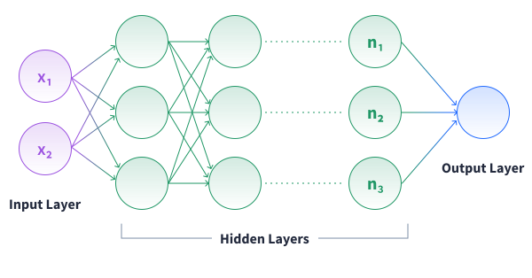
Think of the forward pass like making an educated guess. For example, if we’re trying to predict a person’s salary, the forward pass might take their age and years of experience and spit out a salary estimate. Of course, that guess could be too high or too low—which is where the network learns to adjust itself.
How to Use PyTorch to Predict a Person's Salary
To make this concrete, we’ll walk through an example of how to predict a person’s salary given their age and years of experience. It’s a simplified scenario, but it neatly demonstrates the basics of neural networks—forward pass, loss calculation, and backpropagation.
How the Model Works (Step by Step)
Let’s say we have a single hidden layer with two neurons ($n_1$ and $n_2$) as shown in the image below.
For each neuron, the calculation goes like this:
$$
\begin{align*}
n_1 &= (\text{age} \times w_{1}) + (\text{experience} \times w_{2}) = (24 \times 3) + (5 \times -4) = 52 \\
n_2 &= (\text{age} \times w_{3}) + (\text{experience} \times w_{4}) = (24 \times 1) + (5 \times 2) = 34 \\
\end{align*}
$$
Then these neuron outputs get passed forward to the final output layer to produce a single salary estimate ($y_{est}$):
$$ y_{est} = (n_1 \times w_{5}) + (n_2 \times w_{6}) = (52 \times 2) + (34 \times -1) = 70 $$
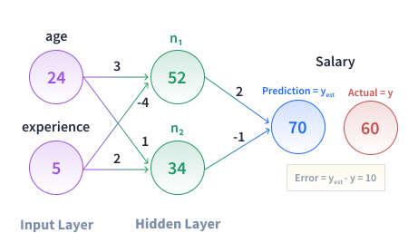
At this point, the model updates its weights by a process known as backpropagation, which we’ll go over in a moment. Notice how the new weights affect the predicted salary—and how the error (difference from the actual salary) has gone down.
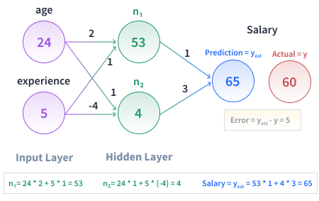
(In reality, these updates don’t always happen in a neat upward-or-downward pattern each time—sometimes the error might temporarily rise. But overall, training should trend toward lower error.)
The Concept of Loss (Error)
Every time the network makes a prediction, we use a loss function to measure how far off we are. For regression tasks (like predicting a continuous salary), a commonly used loss is Mean Squared Error (MSE):
$$ \text{MSE} = \frac{1}{N} \sum_{i=1}^N (y_{\text{est}_i} - y_{\text{act}_i})^2 $$
Here, $N$ is the total number of data points (or people) in the dataset, $i$ indexes each individual from 1 to $N$, $y_{\text{est}_i}$ is the predicted salary for the $i$-th person, and $y_{\text{act}_i}$ is their actual salary.
By squaring the differences between the estimate and the actual value, large errors get penalized more heavily, encouraging the model to aim for more accurate predictions.
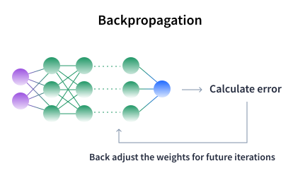
Backpropagation (The Backward Pass)
After computing the loss, the network adjusts weights and biases through backpropagation—a process that calculates how much each parameter contributed to the error and determines how to adjust it to reduce the loss.
An important factor in this adjustment is the learning rate, a hyperparameter that controls the size of the steps taken during each update. Its value typically ranges from 0.0001 to 0.1. A learning rate that’s too high may cause the model to overshoot optimal values, while one that’s too low can make learning very slow. It’s common to start with a learning rate of 0.001 and tweak as necessary.
In PyTorch, once you define your model and loss function, backpropagation (triggered by calling loss.backward()) automatically computes the gradients—numerical values that indicate how much each parameter should change to reduce the error—and the optimizer uses these gradients—scaled by the learning rate—to update the model’s parameters.
Installing and Setting Up PyTorch
Before we dive into coding our salary predictor, let’s make sure you have PyTorch properly installed.
1. Create a Dedicated Environment (Recommended)
If you use conda or Python’s built-in venv, you can create a clean environment to avoid dependency conflicts with other projects. For example:
# From the terminal (command line)
conda create -n pytorch_env python=3.11
conda activate pytorch_env
(Or use venv if you prefer—either is fine!)
2. Install PyTorch
The Official PyTorch “Get Started” Page provides specific commands based on your system (Windows, Mac, Linux) and whether you have a GPU. A simple CPU-only install might look like:
# From the terminal (command line)
pip install torch torchvision torchaudio
CPU vs. GPU: If you have an NVIDIA GPU, select a PyTorch install command that includes CUDA. This speeds up large-scale training but isn’t strictly necessary for small demos.
3. Test Your Installation
Once installed, open a Python shell (or Jupyter Notebook) and try:
import torch

print(torch.__version__)
print("CUDA is available? ->", torch.cuda.is_available())
You should see a version number (e.g., 2.X.X) and a True/False indicating whether PyTorch detects a GPU.
4. Optional Sanity Check
It’s often helpful to run a small tensor operation to confirm PyTorch is working as expected:
x = torch.tensor([1.0, 2.0, 3.0])
print(x * 2)
If it prints tensor([2., 4., 6.]), PyTorch is working fine.
Building a Minimal Salary Predictor in PyTorch
Now let’s construct a bare-bones neural network that models the “age + experience → salary” idea. We’ll keep it as simple as possible. All code below is runnable if you’re following along in a Python file or notebook.
1. Define the Dataset
import torch

# Let's say we have a few data points:
# ages = [40, 22, 55, ...]
# experience = [10, 2, 16, ...]
# salaries = [140, 89, 181, ...] (in thousands)

# We'll define them as Tensors:
ages = torch.tensor([40, 22, 55, 30, 45, 60, 35, 28, 50], dtype=torch.float32)
experience = torch.tensor([10, 2, 16, 6, 12, 18, 8, 4, 14], dtype=torch.float32)
salaries = torch.tensor([140, 89, 181, 113, 154, 194, 127, 104, 167], dtype=torch.float32)

# Now let's combine age & experience into a 2D tensor for convenience:
# Each row will be [age, experience]
inputs = torch.stack((ages, experience), dim=1)

# Normalize the inputs using standard normalization (per feature)
inputs = (inputs - inputs.mean(dim=0)) / inputs.std(dim=0)

# Scale the salaries to a similar range by dividing by 100,
# then convert to a 2D tensor (shape: [num_samples, 1])
targets = (salaries / 100).unsqueeze(1)

print("Inputs shape:", inputs.shape)   # Should be ([9, 2])
print("Targets shape:", targets.shape) # Should be ([9, 1])
Here, we have nine data points. Obviously, this is a tiny dataset—just for demonstration purposes. Typically, you’ll have thousands of data points to help the model learn a pattern.
2. Create a Simple Neural Network
We’ll use a single Linear layer (no hidden layer) to keep things simple:
import torch.nn as nn

# Define a simple linear model with a single layer:
model = nn.Linear(in_features=2, out_features=1)
This layer automatically creates two weights (for age and experience) and a bias term.
3. Define the Loss Function and Optimizer
import torch.optim as optim

# Use Mean Squared Error (MSE) as the loss function
loss_fn = nn.MSELoss()

# Use Stochastic Gradient Descent (SGD) with a moderate learning rate
optimizer = optim.SGD(model.parameters(), lr=0.05)- MSELoss: Perfect for regression, penalizing the square of differences.
- SGD (Stochastic Gradient Descent): Optimizer that adjusts weights based on the gradients. A moderate learning rate (
lr=0.05) ensures we don’t “overshoot” model updates while also speeding up the training process.
4. Training Loop (Forward + Backward)
num_epochs = 50

for epoch in range(num_epochs):
    # 1. Forward pass: compute model predictions on the inputs
    predictions = model(inputs)

    # 2. Compute the loss between predictions and actual targets
    loss = loss_fn(predictions, targets)

    # 3. Clear any previously accumulated gradients
    optimizer.zero_grad()

    # 4. Backward pass: compute gradients based on the loss
    loss.backward()

    # 5. Update the model parameters (weights and bias)
    optimizer.step()

    # Optional: print loss every 5 epochs to track progress
    if (epoch + 1) % 5 == 0:
print(f"Epoch [{epoch+1}/{num_epochs}], Loss: {loss.item():.4f}")Explanation:
- Epoch: One complete pass through the entire training dataset. During each epoch, every data point is processed by the model—going through the forward pass, loss calculation, gradient reset, backward pass, and parameter update. Training over multiple epochs allows the model to gradually refine its predictions.
- Forward Pass: The model multiplies your inputs by its weights, adds the bias, and outputs salary predictions.
- Loss Calculation: Compares those predictions to the actual salaries.
- Gradient Reset: We zero out gradients so they don’t accumulate from previous steps.
- Backward Pass: PyTorch computes how to adjust each weight/bias by analyzing how they contributed to the loss.
- Step: The optimizer moves the parameters in the direction that (hopefully) reduces the loss next time.
After running this code, you should see the loss decrease, indicating the model is learning to approximate the relationship between age, experience, and salary.
5. Evaluating the Result
import numpy as np

# Generate final predictions from the model
# Convert predictions to NumPy for easy viewing
# Multiply by 100 to scale the predictions back to the original salary range
predicted = np.round(model(inputs).detach().numpy() * 100)

print("Final predicted salaries:", predicted.flatten())
print("Actual salaries:         ", salaries.numpy())
You might see something like:
Final predicted salaries: [139.  89. 181. 111. 153. 195. 125. 106. 167.]
Actual salaries:          [140.  89. 181. 113. 154. 194. 127. 104. 167.]
Even if they’re not exact, the predictions should be much closer than the model’s initial guesses—showing that PyTorch has successfully learned from this tiny dataset.
Practical Advice for a Smoother Experience
- Check Your Dimensions: PyTorch expects inputs (X) and targets (y) to have compatible shapes. A common mistake is forgetting to add that extra dimension to target values (i.e.,
(num_samples, 1)and not(num_samples,)). - Start with a Simple Model: Don’t jump into multi-layer architectures right away. A single
nn.Linearcan teach you the fundamentals of forward, backward, and training loops without making things more complex than they need to be. - Go Easy on the Learning Rate: If your loss is bouncing around wildly, you might need to lower the learning rate. If training is crawling, a higher rate could help—but tweak carefully.
- Scale Your Inputs and Targets: Normalizing your inputs and targets (e.g., scaling numerical features to a similar range) can greatly improve training stability. Unscaled features might lead to excessively large gradients and/or unstable learning. Techniques like standard normalization or min-max scaling are recommended.
- GPU or CPU: If you’re working with large datasets or deeper networks, a GPU can drastically reduce training time. See PyTorch’s GPU documentation for how to move your model/data to CUDA.
- Monitor and Debug: Print the loss periodically to see if it’s trending down. If it’s not, double-check your data shapes, your learning rate, and whether you’re zeroing out gradients after each iteration through the training data.
Next Steps & Additional Resources
Now that you’ve built a simple model and watched PyTorch do its magic, you might be wondering where to go next. Here are a few suggestions:
- PyTorch 60-Minute Blitz: A fast-paced introduction that walks you through everything from creating tensors to training a neural network on a classic dataset (like MNIST digits).
- Learn the Basics: If you prefer a more step-by-step approach, this series explores data loading, building models, and more advanced concepts at a methodical pace.
- Explore Real Datasets: Try applying your new skills to a bigger dataset. For instance, check out a dataset on house prices (think
ageof a house,square footage,location index, etc.). Even this small Kaggle dataset can teach you a ton about real-world data cleaning, overfitting, and hyperparameter tuning. - Dive into CNNs or NLP: Convolutional Neural Networks (CNNs) excel at image-related tasks, while Natural Language Processing (NLP) or text-based applications often rely on Recurrent Neural Networks (RNNs) or Transformers. Both can be done in PyTorch with relevant tutorials in the official docs.
Key Terms Recap
Here’s a quick summary of the key concepts we defined in the article:
- Tensor: A multi-dimensional array (similar to a NumPy array) that PyTorch uses to store and process data on both CPUs and GPUs.
- Neural Network: A model made up of layers of neurons, each multiplying inputs by weights and adding biases.
- Forward Pass: The process of sending inputs through the network to get a prediction.
- Loss (or Error): A measurement of how far off predictions are from actual values; lower is better.
- Mean Squared Error (MSE): Squares the difference between predicted and actual values, penalizing large errors more strongly.
- Backpropagation: An algorithm that calculates how to adjust weights and biases based on the loss.
- Gradients: Numerical values computed during backpropagation that indicate how much each parameter (weight or bias) contributes to the error. These values guide how the model should adjust its parameters to minimize the loss.
- Optimizer: An algorithm that uses gradients to update the model's parameters. It determines the step size for each update (often influenced by the learning rate) to help the model converge toward a solution that minimizes the loss.
- Learning Rate: Controls how big a step you take when updating weights. Too large can cause instability; too small can slow training.
- Epoch: One complete pass over your training data—often repeated many times.
Wrapping Up
You’ve just walked through the basics of deep learning with PyTorch, focusing on a concrete example: predicting salaries from just age and experience. We covered:
- Key concepts (layers, forward pass, loss, backprop)
- Why PyTorch is a top choice for modern AI
- Installing and testing PyTorch in a clean environment
- Building a minimal linear model with actual code you can run
- Practical tips to smooth out your learning journey
Remember, every expert started at square one. PyTorch’s strength lies in letting you experiment iteratively—try new architectures, tweak parameters, and see immediate results. As you get comfortable, you’ll find countless avenues to explore: from image recognition to sequence models, natural language programming (NLP), and beyond.
Happy coding, and welcome to the exciting world of PyTorch for deep learning!