DateTime in Pandas: An Uncomplicated Guide
We are surrounded by data that comes in different types and forms. No doubt, one of the most interesting and essential data categories is time-series data. Time-series data is everywhere, and it has many applications across various industries. Patient health metrics, stock price changes, weather records, economic indicators, servers, networks, sensors, and applications performance monitoring are examples of time-series data.
We can define time-series data as a collection of data points obtained at different time intervals and ordered chronologically.
Pandas library basically was developed for analyzing financial time series data and providing a comprehensive framework for working with times, dates, and time-series data.
This tutorial will discuss different aspects of working with dates and times in pandas. After you finish this tutorial, you'll know the following:
- The function of the
TimestampandPeriodobjects - How to work with time-series DataFrames
- How to slice time-series
- The
DateTimeIndexobject and its methods - How to resample time-series data
In this tutorial, we assume you know the fundamentals of pandas Series and DataFrames. If you're not familiar with the pandas library, you might like to try our Pandas and NumPy Fundamentals – Dataquest.
Let's get started.
Exploring Pandas Timestamp and Period Objects
The pandas library provides a DateTime object with nanosecond precision called Timestamp to work with date and time values. The Timestamp object derives from the NumPy's datetime64 data type, making it more accurate and significantly faster than Python's DateTime object. Let's create some Timestamp objects using the Timestamp constructor. Open Jupyter Notebook or VS Code, and run the following code:
import pandas as pd
import numpy as np
from IPython.display import display

print(pd.Timestamp(year=1982, month=9, day=4, hour=1, minute=35, second=10))
print(pd.Timestamp('1982-09-04 1:35.18'))
print(pd.Timestamp('Sep 04, 1982 1:35.18'))
1982-09-04 01:35:10
1982-09-04 01:35:10
1982-09-04 01:35:10Running the code above returns the outputs, which all represent the same instance of time or timestamp.
If you pass a single integer or float value to the Timestamp constructor, it returns a timestamp equivalent to the number of nanoseconds after the Unix epoch (Jan 1, 1970):
print(pd.Timestamp(5000))1970-01-01 00:00:00.000005The Timestamp object inclues many methods and properties that help us access different aspects of a timestamp. Let’s try them:
time_stamp = pd.Timestamp('2022-02-09')
print('{}, {} {}, {}'.format(time_stamp.day_name(), time_stamp.month_name(), time_stamp.day, time_stamp.year))
Wednesday, February 9, 2022While an instance of the Timestamp class represents a single point of time, an instance of the Period object represents a period such as a year, a month, etc.
For example, companies monitor their revenue over a period of a year. Pandas library provides an object called Period to work with periods, as follows:
year = pd.Period('2021')
display(year)
Period('2021', 'A-DEC')You can see here that it creates a Period object representing the year 2021 period, and the 'A-DEC' means that the period is annual, which ends in December.
The Period object provides many useful methods and properties. For example, if you want to return the start and end time of the period, use the following properties:
print('Start Time:', year.start_time)
print('End Time:', year.end_time)
Start Time: 2021-01-01 00:00:00
End Time: 2021-12-31 23:59:59.999999999To create a monthly period, you can pass a specific month to it, as follows:
month = pd.Period('2022-01')
display(month)
print('Start Time:', month.start_time)
print('End Time:', month.end_time)
Period('2022-01', 'M')
Start Time: 2022-01-01 00:00:00
End Time: 2022-01-31 23:59:59.999999999The 'M' indicates that the frequency of the period is monthly. You also can specify the frequency of the period explicitly with the freq argument. The code below creates a period object that represents the period of Jan 1, 2022:
day = pd.Period('2022-01', freq='D')
display(day)
print('Start Time:', day.start_time)
print('End Time:', day.end_time)
Period('2022-01-01', 'D')
Start Time: 2022-01-01 00:00:00
End Time: 2022-01-01 23:59:59.999999999We also can perform arithmetic operations on a period object. Let’s create a new period object with hourly frequency and see how we can do the calculations:
hour = pd.Period('2022-02-09 16:00:00', freq='H')
display(hour)
display(hour + 2)
display(hour - 2)
Period('2022-02-09 16:00', 'H')
Period('2022-02-09 18:00', 'H')
Period('2022-02-09 14:00', 'H')We can get the same results using the pandas date offsets:
display(hour + pd.offsets.Hour(+2))
display(hour + pd.offsets.Hour(-2))
Period('2022-02-09 18:00', 'H')
Period('2022-02-09 14:00', 'H')To create a sequence of dates, you can use the pandas range_dates() method. Let’s try it in the snippet:
week = pd.date_range('2022-2-7', periods=7)
for day in week:
    print('{}-{}\t{}'.format(day.day_of_week, day.day_name(), day.date()))
0-Monday 2022-02-07
1-Tuesday 2022-02-08
2-Wednesday 2022-02-09
3-Thursday 2022-02-10
4-Friday 2022-02-11
5-Saturday 2022-02-12
6-Sunday 2022-02-13The data type of week is a DatetimeIndex object, and each date in the week is an instance of the Timestamp. So we can use all the methods and properties applicable to a Timestamp object.
Creating the Time-Series DataFrame
First, let’s create a DataFrame by reading data from a CSV file containing critical information associated with 50 servers recorded hourly for 34 consecutive days:
df = pd.read_csv('https://raw.githubusercontent.com/m-mehdi/pandas_tutorials/main/server_util.csv')
display(df.head())| datetime | server_id | cpu_utilization | free_memory | session_count | |
|---|---|---|---|---|---|
| 0 | 2019-03-06 00:00:00 | 100 | 0.40 | 0.54 | 52 |
| 1 | 2019-03-06 01:00:00 | 100 | 0.49 | 0.51 | 58 |
| 2 | 2019-03-06 02:00:00 | 100 | 0.49 | 0.54 | 53 |
| 3 | 2019-03-06 03:00:00 | 100 | 0.44 | 0.56 | 49 |
| 4 | 2019-03-06 04:00:00 | 100 | 0.42 | 0.52 | 54 |
Let's look at the content of the DataFrame. Each DataFrame row represents a server's basic performance metrics, including the CPU utilization, free memory, and session count at a specific timestamp. The DataFrame breaks down into one-hour segments. For example, the logged performance metrics from midnight until 4 am are in the first five rows of the DataFrame.
Now, let’s get some details on the characteristics of the DataFrame, such as its size and the data type of each column:
print(df.info())<class 'pandas.core.frame.DataFrame'>
RangeIndex: 40800 entries, 0 to 40799
Data columns (total 5 columns):
# Column Non-Null Count Dtype
--- ------ -------------- -----
0 datetime 40800 non-null object
1 server_id 40800 non-null int64
2 cpu_utilization 40800 non-null float64
3 free_memory 40800 non-null float64
4 session_count 40800 non-null int64
dtypes: float64(2), int64(2), object(1)
memory usage: 1.6+ MB
NoneRunning the statement above returns the number of rows and columns, the total memory usage, the data type of each column, etc.
According to the information above, the data type of the datetime column is an object, which means the timestamps are stored as string values. To convert the data type of the datetime column from a string object to a datetime64 object, we can use the pandas to_datetime() method, as follows:
df['datetime'] = pd.to_datetime(df['datetime'])When we create a DataFrame by importing a CSV file, the date/time values are considered string objects, not DateTime objects. The pandas to_datetime() method converts a date/time value stored in a DataFrame column into a DateTime object. Having date/time values as DateTime objects makes manipulating them much easier. Run the following statement and see the changes:
print(df.info())<class 'pandas.core.frame.DataFrame'>
RangeIndex: 40800 entries, 0 to 40799
Data columns (total 5 columns):
# Column Non-Null Count Dtype
--- ------ -------------- -----
0 datetime 40800 non-null datetime64[ns]
1 server_id 40800 non-null int64
2 cpu_utilization 40800 non-null float64
3 free_memory 40800 non-null float64
4 session_count 40800 non-null int64
dtypes: datetime64[ns](1), float64(2), int64(2)
memory usage: 1.6 MB
NoneNow, the data type of the datetime column is a datetime64[ns]object. The [ns] means the nano second-based time format that specifies the precision of the DateTime object.
Also, we can let the pandas read_csv() method parse certain columns as DataTime objects, which is more straightforward than using the to_datetime() method. Let's try it:
df = pd.read_csv('https://raw.githubusercontent.com/m-mehdi/pandas_tutorials/main/server_util.csv', parse_dates=['datetime'])
print(df.head())
datetime server_id cpu_utilization free_memory session_count
0 2019-03-06 00:00:00 100 0.40 0.54 52
1 2019-03-06 01:00:00 100 0.49 0.51 58
2 2019-03-06 02:00:00 100 0.49 0.54 53
3 2019-03-06 03:00:00 100 0.44 0.56 49
4 2019-03-06 04:00:00 100 0.42 0.52 54Running the code above creates a DataFrame where the data type of the datetime column is a DateTime object.
Before heading to the next section, let’s apply some basic methods to the datetime column.
First, let’s see how we can return the earliest and latest dates in the DataFrame. To do this, we can simply apply the max() and min() methods on the datetime column, as follows:
display(df.datetime.min())
display(df.datetime.max())
Timestamp('2019-03-06 00:00:00')
Timestamp('2019-04-08 23:00:00')To select the DataFrame rows between two specific dates, we can create a Boolean mask and use the .loc method to filter rows within a certain date range:
mask = (df.datetime >= pd.Timestamp('2019-03-06')) & (df.datetime < pd.Timestamp('2019-03-07'))
display(df.loc[mask])| datetime | server_id | cpu_utilization | free_memory | session_count | |
|---|---|---|---|---|---|
| 0 | 2019-03-06 00:00:00 | 100 | 0.40 | 0.54 | 52 |
| 1 | 2019-03-06 01:00:00 | 100 | 0.49 | 0.51 | 58 |
| 2 | 2019-03-06 02:00:00 | 100 | 0.49 | 0.54 | 53 |
| 3 | 2019-03-06 03:00:00 | 100 | 0.44 | 0.56 | 49 |
| 4 | 2019-03-06 04:00:00 | 100 | 0.42 | 0.52 | 54 |
| ... | ... | ... | ... | ... | ... |
| 40003 | 2019-03-06 19:00:00 | 149 | 0.74 | 0.24 | 81 |
| 40004 | 2019-03-06 20:00:00 | 149 | 0.73 | 0.23 | 81 |
| 40005 | 2019-03-06 21:00:00 | 149 | 0.79 | 0.29 | 83 |
| 40006 | 2019-03-06 22:00:00 | 149 | 0.73 | 0.29 | 82 |
| 40007 | 2019-03-06 23:00:00 | 149 | 0.75 | 0.24 | 84 |
1200 rows × 5 columns
Slicing Time Series
To make Timestamp slicing possible, we need to set the datetime column as the index of the DataFrame. To set a column as an index of a DataFrame, use the set_index method:
df.set_index('datetime', inplace=True)
print(df)
datetime server_id cpu_utilization free_memory session_count
2019-03-06 00:00:00 100 0.40 0.54 52
2019-03-06 01:00:00 100 0.49 0.51 58
2019-03-06 02:00:00 100 0.49 0.54 53
2019-03-06 03:00:00 100 0.44 0.56 49
2019-03-06 04:00:00 100 0.42 0.52 54
... ... ... ... ...
2019-04-08 19:00:00 149 0.73 0.20 81
2019-04-08 20:00:00 149 0.75 0.25 83
2019-04-08 21:00:00 149 0.80 0.26 82
2019-04-08 22:00:00 149 0.75 0.29 82
2019-04-08 23:00:00 149 0.75 0.24 80
[40800 rows x 4 columns]To select all the rows equal to a single index using the .loc method:
print(df.loc['2019-03-07 02:00:00'].head(5)) datetime server_id cpu_utilization free_memory session_count
2019-03-07 02:00:00 100 0.44 0.50 56
2019-03-07 02:00:00 101 0.78 0.21 87
2019-03-07 02:00:00 102 0.75 0.27 80
2019-03-07 02:00:00 103 0.76 0.28 85
2019-03-07 02:00:00 104 0.74 0.24 77You can select the rows that partially match a specific Timestamp in the index column. Let’s try it:
print(df.loc['2019-03-07'].head(5)) datetime server_id cpu_utilization free_memory session_count
2019-03-07 00:00:00 100 0.51 0.52 55
2019-03-07 01:00:00 100 0.46 0.50 49
2019-03-07 02:00:00 100 0.44 0.50 56
2019-03-07 03:00:00 100 0.45 0.52 51
2019-03-07 04:00:00 100 0.42 0.50 53The selection string can be any standard date format, let’s look at some examples:
df.loc['Apr 2019']
df.loc['8th April 2019']
df.loc['April 05, 2019 5pm']
We can also use the .loc method to slice rows within a date range. The following statement will return all the rows starting from April 3, 2019, through the end of April 4, 2019; both start and end dates are inclusive:
display(df.loc['03-04-2019':'04-04-2019'])But running it will raise a future warning that is annoying. To get rid of the warning, we can sort the index before slicing rows:
display(df.sort_index().loc['03-04-2019':'04-04-2019'])| datetime | server_id | cpu_utilization | free_memory | session_count |
|---|---|---|---|---|
| 2019-03-06 00:00:00 | 100 | 0.40 | 0.54 | 52 |
| 2019-03-06 00:00:00 | 135 | 0.50 | 0.55 | 55 |
| 2019-03-06 00:00:00 | 110 | 0.54 | 0.40 | 61 |
| 2019-03-06 00:00:00 | 136 | 0.58 | 0.40 | 64 |
| 2019-03-06 00:00:00 | 109 | 0.57 | 0.41 | 61 |
| ... | ... | ... | ... | ... |
| 2019-04-04 23:00:00 | 143 | 0.43 | 0.52 | 50 |
| 2019-04-04 23:00:00 | 111 | 0.53 | 0.52 | 59 |
| 2019-04-04 23:00:00 | 149 | 0.75 | 0.24 | 85 |
| 2019-04-04 23:00:00 | 138 | 0.40 | 0.56 | 47 |
| 2019-04-04 23:00:00 | 107 | 0.63 | 0.33 | 73 |
36000 rows × 4 columns
The DateTimeIndex Methods
Some pandas DataFrame methods are only applicable on the DateTimeIndex. We'll look at some of them in this section, but first, let's make sure our DataFrame has a DateTimeIndex:
print(type(df.index))<class 'pandas.core.indexes.datetimes.DatetimeIndex'>To return the server monitoring data collected at a specific time, regardless of the date, use the at_time() method:
display(df.at_time('09:00'))| datetime | server_id | cpu_utilization | free_memory | session_count |
|---|---|---|---|---|
| 2019-03-06 09:00:00 | 100 | 0.48 | 0.51 | 51 |
| 2019-03-07 09:00:00 | 100 | 0.45 | 0.49 | 56 |
| 2019-03-08 09:00:00 | 100 | 0.45 | 0.53 | 53 |
| 2019-03-09 09:00:00 | 100 | 0.45 | 0.51 | 53 |
| 2019-03-10 09:00:00 | 100 | 0.49 | 0.55 | 55 |
| ... | ... | ... | ... | ... |
| 2019-04-04 09:00:00 | 149 | 0.75 | 0.21 | 80 |
| 2019-04-05 09:00:00 | 149 | 0.71 | 0.26 | 83 |
| 2019-04-06 09:00:00 | 149 | 0.75 | 0.30 | 83 |
| 2019-04-07 09:00:00 | 149 | 0.81 | 0.28 | 77 |
| 2019-04-08 09:00:00 | 149 | 0.82 | 0.24 | 86 |
1700 rows × 4 columns
Also, to select all the server data between midnight and 2 AM on all dates, use the between_time() method. Let's try it:
display(df.between_time('00:00','02:00'))| datetime | server_id | cpu_utilization | free_memory | session_count |
|---|---|---|---|---|
| 2019-03-06 00:00:00 | 100 | 0.40 | 0.54 | 52 |
| 2019-03-06 01:00:00 | 100 | 0.49 | 0.51 | 58 |
| 2019-03-06 02:00:00 | 100 | 0.49 | 0.54 | 53 |
| 2019-03-07 00:00:00 | 100 | 0.51 | 0.52 | 55 |
| 2019-03-07 01:00:00 | 100 | 0.46 | 0.50 | 49 |
| ... | ... | ... | ... | ... |
| 2019-04-07 01:00:00 | 149 | 0.74 | 0.21 | 78 |
| 2019-04-07 02:00:00 | 149 | 0.76 | 0.26 | 74 |
| 2019-04-08 00:00:00 | 149 | 0.75 | 0.28 | 75 |
| 2019-04-08 01:00:00 | 149 | 0.69 | 0.27 | 79 |
| 2019-04-08 02:00:00 | 149 | 0.78 | 0.20 | 85 |
5100 rows × 4 columns
We can use the first() method to select the first DataFrame rows based on a specific date offset. For instance, passing 5B as a date offset to the method returns all the rows with indices within the first five business days. Similarly, passing 1W to the last() method returns all the DataFrame rows with indices within the last week. Notice that the DataFrame must be sorted on its index to ensure these methods work. Let's try both examples:
display(df.sort_index().first('5B'))| datetime | server_id | cpu_utilization | free_memory | session_count |
|---|---|---|---|---|
| 2019-03-06 | 100 | 0.40 | 0.54 | 52 |
| 2019-03-06 | 135 | 0.50 | 0.55 | 55 |
| 2019-03-06 | 110 | 0.54 | 0.40 | 61 |
| 2019-03-06 | 136 | 0.58 | 0.40 | 64 |
| 2019-03-06 | 109 | 0.57 | 0.41 | 61 |
| ... | ... | ... | ... | ... |
| 2019-03-12 | 134 | 0.53 | 0.45 | 61 |
| 2019-03-12 | 144 | 0.68 | 0.31 | 73 |
| 2019-03-12 | 113 | 0.76 | 0.24 | 83 |
| 2019-03-12 | 114 | 0.58 | 0.48 | 67 |
| 2019-03-12 | 131 | 0.58 | 0.42 | 67 |
7250 rows × 4 columns
display(df.sort_index().last('1W'))| datetime | server_id | cpu_utilization | free_memory | session_count |
|---|---|---|---|---|
| 2019-04-08 00:00:00 | 106 | 0.44 | 0.62 | 49 |
| 2019-04-08 00:00:00 | 112 | 0.72 | 0.29 | 81 |
| 2019-04-08 00:00:00 | 100 | 0.43 | 0.54 | 51 |
| 2019-04-08 00:00:00 | 137 | 0.75 | 0.28 | 83 |
| 2019-04-08 00:00:00 | 110 | 0.61 | 0.40 | 62 |
| ... | ... | ... | ... | ... |
| 2019-04-08 23:00:00 | 128 | 0.64 | 0.41 | 64 |
| 2019-04-08 23:00:00 | 127 | 0.67 | 0.33 | 78 |
| 2019-04-08 23:00:00 | 126 | 0.71 | 0.33 | 73 |
| 2019-04-08 23:00:00 | 123 | 0.71 | 0.22 | 83 |
| 2019-04-08 23:00:00 | 149 | 0.75 | 0.24 | 80 |
1200 rows × 4 columns
df.sort_index().last('2W')| datetime | server_id | cpu_utilization | free_memory | session_count |
|---|---|---|---|---|
| 2019-04-01 00:00:00 | 120 | 0.54 | 0.48 | 63 |
| 2019-04-01 00:00:00 | 104 | 0.73 | 0.31 | 83 |
| 2019-04-01 00:00:00 | 103 | 0.77 | 0.22 | 82 |
| 2019-04-01 00:00:00 | 124 | 0.39 | 0.55 | 49 |
| 2019-04-01 00:00:00 | 127 | 0.68 | 0.37 | 73 |
| ... | ... | ... | ... | ... |
| 2019-04-08 23:00:00 | 128 | 0.64 | 0.41 | 64 |
| 2019-04-08 23:00:00 | 127 | 0.67 | 0.33 | 78 |
| 2019-04-08 23:00:00 | 126 | 0.71 | 0.33 | 73 |
| 2019-04-08 23:00:00 | 123 | 0.71 | 0.22 | 83 |
| 2019-04-08 23:00:00 | 149 | 0.75 | 0.24 | 80 |
9600 rows × 4 columns
Resampling Time Series Data
The logic behind the resample() method is similar to the groupby() method. It groups data within any possible period. Although we can use the resample() method for both upsampling and downsampling, we'll focus on how to use it to perform downsampling, which reduces the frequency of time-series data — for instance, converting hourly time-series data to daily or daily time-series data to monthly.
The following example returns the average CPU utilization, free memory, and active session count of server ID 100 each day. To do that, we need first to filter the DataFrame's rows with server ID 100, then we resample the hourly data to daily data. Finally, apply the mean() method on the result to get the daily average of the three metrics:
df[df.server_id == 100].resample('D')['cpu_utilization', 'free_memory', 'session_count'].mean()| datetime | cpu_utilization | free_memory | session_count |
|---|---|---|---|
| 2019-03-06 | 0.470417 | 0.535417 | 53.000000 |
| 2019-03-07 | 0.455417 | 0.525417 | 53.666667 |
| 2019-03-08 | 0.478333 | 0.532917 | 54.541667 |
| 2019-03-09 | 0.472917 | 0.523333 | 54.166667 |
| 2019-03-10 | 0.465000 | 0.527500 | 54.041667 |
| 2019-03-11 | 0.469583 | 0.528750 | 53.916667 |
| 2019-03-12 | 0.475000 | 0.533333 | 53.750000 |
| 2019-03-13 | 0.462917 | 0.521667 | 52.541667 |
| 2019-03-14 | 0.472083 | 0.532500 | 54.875000 |
| 2019-03-15 | 0.470417 | 0.530417 | 53.500000 |
| 2019-03-16 | 0.463750 | 0.530833 | 54.416667 |
| 2019-03-17 | 0.472917 | 0.532917 | 52.041667 |
| 2019-03-18 | 0.475417 | 0.535000 | 53.333333 |
| 2019-03-19 | 0.460833 | 0.546667 | 54.791667 |
| 2019-03-20 | 0.467083 | 0.529167 | 54.375000 |
| 2019-03-21 | 0.465833 | 0.543333 | 54.375000 |
| 2019-03-22 | 0.468333 | 0.528333 | 54.083333 |
| 2019-03-23 | 0.462500 | 0.539167 | 53.916667 |
| 2019-03-24 | 0.467917 | 0.537917 | 54.958333 |
| 2019-03-25 | 0.461250 | 0.530000 | 54.000000 |
| 2019-03-26 | 0.456667 | 0.531250 | 54.166667 |
| 2019-03-27 | 0.466667 | 0.530000 | 53.291667 |
| 2019-03-28 | 0.468333 | 0.532083 | 53.291667 |
| 2019-03-29 | 0.472917 | 0.538750 | 53.541667 |
| 2019-03-30 | 0.463750 | 0.526250 | 54.458333 |
| 2019-03-31 | 0.465833 | 0.522500 | 54.833333 |
| 2019-04-01 | 0.468333 | 0.527083 | 53.333333 |
| 2019-04-02 | 0.464583 | 0.515000 | 53.708333 |
| 2019-04-03 | 0.472500 | 0.533333 | 54.583333 |
| 2019-04-04 | 0.472083 | 0.531250 | 53.291667 |
| 2019-04-05 | 0.451250 | 0.540000 | 53.833333 |
| 2019-04-06 | 0.464167 | 0.531250 | 53.750000 |
| 2019-04-07 | 0.472500 | 0.530417 | 54.541667 |
| 2019-04-08 | 0.464583 | 0.534167 | 53.875000 |
We can also view the same result for every server ID by chaining the groupby() and resample() methods.
The following statement returns the maximum CPU utilization and free memory each month for each server. Let's try it:
df.groupby(df.server_id).resample('M')['cpu_utilization', 'free_memory'].max()| server_id | datetime | cpu_utilization | free_memory |
|---|---|---|---|
| 100 | 2019-03-31 | 0.56 | 0.62 |
| 2019-04-30 | 0.55 | 0.61 | |
| 101 | 2019-03-31 | 0.91 | 0.32 |
| 2019-04-30 | 0.89 | 0.30 | |
| 102 | 2019-03-31 | 0.85 | 0.36 |
| ... | ... | ... | ... |
| 147 | 2019-04-30 | 0.61 | 0.57 |
| 148 | 2019-03-31 | 0.84 | 0.35 |
| 2019-04-30 | 0.83 | 0.34 | |
| 149 | 2019-03-31 | 0.85 | 0.36 |
| 2019-04-30 | 0.83 | 0.34 |
100 rows × 2 columns
Before we conclude this tutorial, let's plot the average CPU utilization of each server on a monthly basis. The result gives us enough visibility on the changing of the average CPU utilization of each server over months.
import matplotlib.pyplot as plt

fig, ax = plt.subplots(figsize=(24, 8))
df.groupby(df.server_id).resample('M')['cpu_utilization'].mean()\
.plot.bar(color=['green', 'gray'], ax=ax, title='The Average Monthly CPU Utilization Comparison')
<AxesSubplot:title={'center':'The Average Monthly CPU Utilization Comparison'}, xlabel='server_id,datetime'>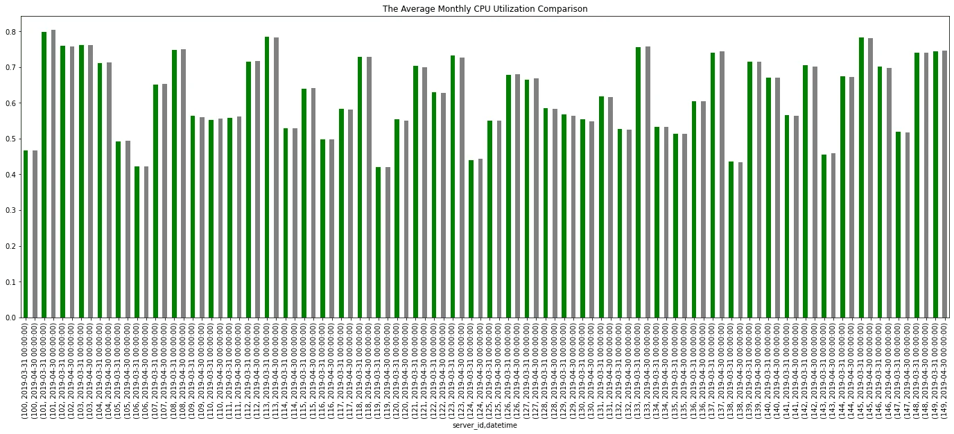
Conclusion
Pandas is an excellent analytical tool, especially when it comes to dealing with time-series data. The library provides extensive tools for working with time-indexed DataFrames. This tutorial covered the essential aspects of working with date and time in pandas.
If you’d like to learn more about working with time-series data in pandas, you can check out the Time Series Analysis with Pandas tutorial on the Dataquest blog, and of course, the Pandas documentation on Time series / date functionality.