Working with RDDs in PySpark

In the previous tutorial, you saw how to set up PySpark locally and got your first taste of SparkSession, the modern entry point that coordinates Spark's distributed processing. You saw how the Driver orchestrates Executors across a cluster, and you experienced lazy evaluation firsthand when operations didn't execute until you called an action.

Now it's time to go deeper into working with RDDs. To make this tutorial hands-on and practical, we'll work with real-world population data sourced from Wikipedia's list of countries by population. This CSV dataset contains country names, population counts, percentages of world population, and update dates. We'll use it to explore how RDDs handle structured data at scale.

By the end of this tutorial, you'll understand:

• What makes RDDs "resilient and distributed" within the SparkSession ecosystem
• The difference between transformations and actions in PySpark
• How to create and manipulate RDDs using core operations
• How Directed Acyclic Graphs (DAGs) optimize your data processing pipeline
• When RDDs are still the right choice for modern data science workflows

Let's start by understanding what exactly makes an RDD the foundation of Spark's distributed computing power.

What Are RDDs?

Resilient Distributed Datasets (RDDs) are Spark's original data structure for distributed computing. Think of an RDD as a very large Python list that's been:

• Split into partitions and distributed across multiple machines or CPU cores
• Stored in memory for fast access during processing
• Made fault-tolerant through automatic rebuilding if any partition fails

As you learned in the previous tutorial, SparkSession is your unified entry point to all Spark functionality. While SparkSession gives you access to higher-level abstractions like DataFrames and SQL, it also provides seamless access to RDD operations through its underlying SparkContext.

Why Learn RDDs When DataFrames Exist?

While DataFrames handle most of your day-to-day data tasks, understanding Resilient Distributed Datasets (RDDs) gives you the foundation to work with Spark's core execution model. RDDs are Spark's original data abstraction. They’re the building blocks that made distributed computing accessible to Python developers.

But you may wonder: "If DataFrames are more optimized and easier to use, why learn RDDs?" And it’s a great question. Here's why RDDs remain valuable:

RDDs excel when you need:

• Fine-grained control over data distribution and processing
• Custom transformations that don't map well to SQL-like operations
• Machine learning algorithms that require iterative processing
• Streaming data processing with complex event handling

DataFrames are better for:

• Structured data with known schemas
• SQL-like operations (filtering, grouping, joining)
• Automatic optimizations for query performance
• Integration with Spark SQL and MLlib

For this tutorial, we'll focus on RDD fundamentals through practical examples.

Let's start by loading our population dataset and exploring how RDDs work.

Loading Data with RDDs

Using our familiar SparkSession setup:

import os
import sys
from pyspark.sql import SparkSession

# Ensure PySpark uses the same Python interpreter as this script
os.environ["PYSPARK_PYTHON"] = sys.executable

# Create SparkSession
spark = SparkSession.builder \
    .appName("RDD_PopulationAnalysis") \
    .master("local[*]") \
    .config("spark.driver.memory", "2g") \
    .getOrCreate()

# Load data through SparkSession's SparkContext
population_rdd = spark.sparkContext.textFile("world_population.csv")
sample_data = population_rdd.take(3)
print("Sample data from population dataset:")
for line in sample_data:
    print(line)

print(f"\nRDD type:    {type(population_rdd)}")
print(f"Sample type: {type(sample_data)}")

Sample data from population dataset:
location,population,percent_of_world,date_updated
India,1413324000,17.3%,1 Mar 2025
China,1408280000,17.2%,31 Dec 2024

RDD type:    <class 'pyspark.core.rdd.RDD'>
Sample type: <class 'list'>

Let's break down what's happening in this code:

SparkSession Configuration:

• .appName("RDD_PopulationAnalysis") gives our Spark application a descriptive name
• .master("local[*]") runs Spark locally using all available CPU cores
• .config("spark.driver.memory", "2g") allocates 2GB of memory for the driver process

Loading and Sampling Data:

• spark.sparkContext.textFile() creates an RDD where each line becomes one element
• .take(3) returns the first 3 elements as a regular Python list

Did you notice something important? We iterated over sample_data (the result from .take(3)), not over population_rdd directly. That's because RDDs aren't iterable like Python lists, since their data is distributed across multiple machines or cores. To work with RDD contents, we need to use Spark actions that either return Python objects or trigger distributed computation.

Transformations vs Actions: The Heart of Spark Programming

The distinction between transformations and actions is fundamental to writing efficient PySpark code. We touched on this previously when we talked about lazy evaluation, but now let's explore it thoroughly.

Transformations: Building Your Data Pipeline

Transformations are operations that define what you want to do with your data, but they don't execute immediately. Instead, they build a computation plan that Spark will optimize and execute later.

When you need to load data from files, use:

• .textFile(): Load text data from files into an RDD

When you need to transform each element, use:

• .map(): Apply a function to each element in the RDD

When you need to filter data based on conditions, use:

• .filter(): Keep only elements that meet certain criteria

Let's see these transformations in action:

# These are all transformations - they build a plan but don't execute
header_removed = population_rdd.filter(lambda line: not line.startswith("location"))
split_lines = header_removed.map(lambda line: line.split(","))
countries_only = split_lines.map(lambda fields: (fields[0], int(fields[1])))

print("Transformations created:")
print(f"Original RDD: {population_rdd}")
print(f"After filter: {header_removed}")
print(f"After map: {split_lines}")
print(f"After final map: {countries_only}")
print("\nNo data has been processed yet - these are just execution plans!")

Transformations created:
Original RDD: world_population.csv MapPartitionsRDD[1] at textFile at NativeMethodAccessorImpl.java:0
After filter: PythonRDD[2] at RDD at PythonRDD.scala:53
After map: PythonRDD[3] at RDD at PythonRDD.scala:53
After final map: PythonRDD[4] at RDD at PythonRDD.scala:53

No data has been processed yet - these are just execution plans!

Each transformation creates a new RDD object with a reference like PythonRDD[2], PythonRDD[3], etc. The number in square brackets is Spark's internal ID for tracking different RDDs in your application—each new transformation gets the next sequential number. These aren't data, they're execution plans waiting to be triggered.

Actions: Triggering Computation and Returning Results

Actions are operations that force Spark to execute your transformation pipeline and return results. Unlike transformations that return RDDs, actions return regular Python objects.

When you need to inspect your data, use:

• .take(n): Return the first n elements as a Python list
• .first(): Return the first element as a Python object

When you need to collect results, use:

• .collect(): Return all elements as a Python list (use carefully!)

When you need to count elements, use:

• .count(): Return the number of elements as a Python integer

When you need to aggregate data, use:

• .reduce(): Combine elements using a function, return a single Python object

Let's trigger our transformation pipeline with an action:

# This action triggers execution of the entire transformation chain
# Note: .take() returns a regular Python list, not an RDD
result = countries_only.take(5)
print("Now the transformations execute!")
print(f"Result type: {type(result)}")  # This will be a Python list
print("Country-population pairs:")
for country, population in result:
    print(f"{country}: {population:,}")

Now the transformations execute!
Result type: <class 'list'>
Country-population pairs:
India: 1,413,324,000
China: 1,408,280,000
United States: 340,110,988
Indonesia: 282,477,584
Pakistan: 241,499,431

Only when we called .take(5) did Spark actually execute the pipeline and return a regular Python list. This is just lazy evaluation at work.

The key pattern to remember: transformations return RDDs, actions return Python objects. This is why .collect() is so useful; it converts your distributed RDD into a regular Python list that you can iterate over normally. However, avoid using .collect() on large datasets since it loads everything into memory at once. Filtering your data first can help a lot.

(Note: Some actions like .saveAsTextFile() return nothing after writing to disk.)

Understanding DAGs: Spark's Optimization Engine

When you chain transformations together, Spark creates a Directed Acyclic Graph (DAG) that represents your computation. A DAG is a network of connected nodes where:

• Nodes represent operations (like map, filter, or data sources)
• Directed edges show the flow of data from one operation to the next
• Acyclic means there are no circular dependencies because data flows in one direction

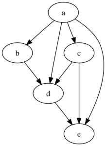
Looking at the diagram above, you can see how node 'a' flows to nodes 'b' and 'c' (amongst others), which both contribute to node 'd', and finally it flows to node 'e'. In Spark terms, this might represent: load data (a) → filter (b) and map (c) → join results (d) → final output (e).

This DAG structure allows Spark to:

• Combine operations for efficiency (e.g., filter + map = single pass through data)
• Minimize data movement between machines
• Recover from failures by rebuilding only necessary partitions
• Optimize resource usage across the cluster

Let's create a more complex transformation pipeline to see DAG optimization at work:

# Complex transformation chain
processed_data = population_rdd \
    .filter(lambda line: not line.startswith("location")) \
    .map(lambda line: line.split(",")) \
    .filter(lambda fields: len(fields) >= 2) \
    .map(lambda fields: (fields[0], int(fields[1]))) \
    .filter(lambda pair: pair[1] > 100_000_000)

print("Complex transformation chain created")
print(f"Final RDD: {processed_data}")
print("Spark has built a DAG to optimize this pipeline")

# Trigger execution and get a Python list
large_countries = processed_data.collect()  # Returns Python list
print(f"\nResult type: {type(large_countries)}")
print(f"Countries with population > 100 million:")
for country, population in large_countries[:10]:  # Now we can iterate normally
    print(f"{country}: {population:,}")

Complex transformation chain created
Final RDD: PythonRDD[8] at RDD at PythonRDD.scala:53
Spark has built a DAG to optimize this pipeline

Result type: <class 'list'>
Countries with population > 100 million:
India: 1,413,324,000
China: 1,408,280,000
United States: 340,110,988
Indonesia: 282,477,584
Pakistan: 241,499,431
Nigeria: 223,800,000
Brazil: 212,583,750
Bangladesh: 169,828,911
Russia: 146,028,325
Mexico: 130,417,144

Let's break down this transformation chain:

1. .filter(lambda line: not line.startswith("location")) - Remove the CSV header row
2. .map(lambda line: line.split(",")) - Split each line into a list of fields
3. .filter(lambda fields: len(fields) >= 2) - Keep only rows with at least 2 columns (data quality check)
4. .map(lambda fields: (fields[0], int(fields[1]))) - Create tuples of (country_name, population_as_integer)
5. .filter(lambda pair: pair[1] > 100_000_000) - Keep only countries with population over 100 million

Each transformation adds a step to Spark's execution plan, building up a processing pipeline that won't execute until we call an action. Behind the scenes, Spark optimizes this chain by pipelining operations and planning efficient execution, all before running a single step! (With DataFrames, these optimizations get even more sophisticated.)

Hands-On: Population Data Analysis with RDDs

Now let's put these concepts into practice with a comprehensive analysis of our world population data. We'll work through the complete data processing pipeline, from loading raw data to computing meaningful insights.

Task 1: Load and Explore the Dataset Structure

First, we need to understand what we're working with. For this task, we'll use the .take() action to get a sample and the .count() action to understand the dataset size.

# Examine the first few lines (action - returns Python list)
sample_lines = population_rdd.take(5)
print("Raw data sample:")
for i, line in enumerate(sample_lines):
    print(f"Line {i}: {line}")

# Check total number of lines (action - returns Python integer)
total_lines = population_rdd.count()
print(f"\nTotal lines in dataset: {total_lines}")
print(f"Sample type: {type(sample_lines)}")  # Python list
print(f"Count type: {type(total_lines)}")    # Python integer

Raw data sample:
Line 0: location,population,percent_of_world,date_updated
Line 1: India,1413324000,17.3%,1 Mar 2025
Line 2: China,1408280000,17.2%,31 Dec 2024
Line 3: United States,340110988,4.2%,1 Jul 2024
Line 4: Indonesia,282477584,3.5%,30 Jun 2024

Total lines in dataset: 240
Sample type: <class 'list'>
Count type: <class 'int'>

Our dataset contains 240 lines, including the header. Notice how the actions return regular Python objects that we can work with normally.

Task 2: Remove Headers from Raw Data

Next, we need to clean our data by removing the header row. For this task, we'll use the .first() action to identify the header and the .filter() transformation to exclude it.

# Get the header line (action - returns Python string)
header = population_rdd.first()
print(f"Header: {header}")
print(f"Header type: {type(header)}")  # Python string

# Remove header from dataset (transformation - returns new RDD)
data_without_header = population_rdd.filter(lambda line: line != header)

# Verify header removal (action - returns Python list)
verification_sample = data_without_header.take(3)
print("\nData after header removal:")
for line in verification_sample:
    print(line)

# Count remaining lines (action - returns Python integer)
data_count = data_without_header.count()
print(f"\nLines after header removal: {data_count}")

Header: location,population,percent_of_world,date_updated
Header type: <class 'str'>

Data after header removal:
India,1413324000,17.3%,1 Mar 2025
China,1408280000,17.2%,31 Dec 2024
United States,340110988,4.2%,1 Jul 2024

Lines after header removal: 239

Perfect! We've successfully removed the header and confirmed we have 239 countries in our dataset.

Task 3: Parse Raw Text into Structured Data

Now we need to convert our raw CSV strings into structured data we can analyze. For this task, we'll use the .map() transformation to split and restructure each line.

# Split each line into fields (transformation - returns new RDD)
split_data = data_without_header.map(lambda line: line.split(","))

# Check the structure (action - returns Python list)
sample_split = split_data.take(3)
print("Parsed data structure:")
for i, fields in enumerate(sample_split):
    print(f"Country {i+1}: {fields}")

# Transform into structured tuples (transformation - returns new RDD)
structured_data = split_data.map(lambda fields: (
    fields[0],                   # country name
    int(fields[1]),              # population as integer
    fields[2],                   # percentage (keeping as string for now)
    fields[3]                    # date
))

# Verify the transformation (action - returns Python list)
sample_structured = structured_data.take(3)
print("\nStructured data:")
for country, pop, pct, date in sample_structured:
    print(f"{country}: {pop:,} people ({pct}) - updated {date}")

Parsed data structure:
Country 1: ['India', '1413324000', '17.3%', '1 Mar 2025']
Country 2: ['China', '1408280000', '17.2%', '31 Dec 2024']
Country 3: ['United States', '340110988', '4.2%', '1 Jul 2024']

Structured data:
India: 1,413,324,000 people (17.3%) - updated 1 Mar 2025
China: 1,408,280,000 people (17.2%) - updated 31 Dec 2024
United States: 340,110,988 people (4.2%) - updated 1 Jul 2024

Excellent! Our data is now properly structured with population values converted to integers for mathematical operations.

Task 4: Filter Data Based on Population Thresholds

Let's find countries that meet specific population criteria. For this task, we'll use the .filter() transformation to select countries and the .collect() action to gather results.

# Create a simplified RDD with just country and population (transformation)
country_population = structured_data.map(lambda record: (record[0], record[1]))

# Find countries with population over 100 million (transformation)
large_countries = country_population.filter(lambda pair: pair[1] >= 100_000_000)

# Count how many large countries there are (action - returns Python integer)
large_country_count = large_countries.count()
print(f"Countries with population >= 100 million: {large_country_count}")

# Get the complete list (action - returns Python list)
large_countries_list = large_countries.collect()
print(f"\nResult type: {type(large_countries_list)}")
print("Large countries (>=100M population):")
for country, population in large_countries_list:
    print(f"{country}: {population:,}")

Countries with population >= 100 million: 16

Result type: <class 'list'>
Large countries (>=100M population):
India: 1,413,324,000
China: 1,408,280,000
United States: 340,110,988
Indonesia: 282,477,584
Pakistan: 241,499,431
Nigeria: 223,800,000
Brazil: 212,583,750
Bangladesh: 169,828,911
Russia: 146,028,325
Mexico: 130,417,144
Japan: 123,340,000
Philippines: 114,123,600
Ethiopia: 109,499,000
Democratic Republic of the Congo: 109,276,000
Egypt: 107,271,260
Vietnam: 101,343,800

We have 16 countries with populations of 100 million or more. Notice how we used transformations (.map() and .filter()) to build our processing pipeline, then actions (.count() and .collect()) to actually execute the computation and retrieve results.

Task 5: Compute Global Population Statistics

Now let's calculate summary statistics across all countries. For this task, we'll use the .reduce() action to perform custom aggregations. This method works by combining elements two at a time using a function you provide, continuing until only one result remains.

# Extract just the population values (transformation)
populations = country_population.map(lambda pair: pair[1])

# Calculate total world population (action - returns Python integer)
total_population = populations.reduce(lambda x, y: x + y)
print(f"Total world population: {total_population:,}")

# Find the maximum population (action - returns Python integer)
max_population = populations.reduce(lambda x, y: max(x, y))
print(f"Largest country population: {max_population:,}")

# Find the minimum population (action - returns Python integer)
min_population = populations.reduce(lambda x, y: min(x, y))
print(f"Smallest country population: {min_population:,}")

# Calculate average population (combining actions)
country_count = populations.count()  # Action - returns Python integer
average_population = total_population / country_count
print(f"Average country population: {average_population:,.0f}")

print(f"\nAll results are Python objects:")
print(f"Total type: {type(total_population)}")
print(f"Max type: {type(max_population)}")
print(f"Count type: {type(country_count)}")

Total world population: 7,982,296,746
Largest country population: 1,413,324,000
Smallest country population: 35
Average country population: 33,398,731

All results are Python objects:
Total type: <class 'int'>
Max type: <class 'int'>
Count type: <class 'int'>

These statistics reveal the extreme inequality in global population distribution. While the average country has about 33 million people, the largest country (India) has over 1.4 billion while the smallest has just 35 people. This massive range shows why understanding your data distribution matters before applying analytics.

Notice that all our results are regular Python integers returned by actions, ready for further calculations or analysis. Population totals may vary from other sources since official statistics are constantly updated with new estimates and projections.

Task 6: Analyze Population Distribution by Categories

Let's explore how countries are distributed across different population ranges. For this task, we'll use .map() for categorization and .reduceByKey() for counting. The .reduceByKey() transformation works specifically with key-value pair RDDs, grouping all pairs that share the same key and then combining their values using a function you provide.

# Categorize countries by population size (transformation)
def categorize_population(population):
    if population >= 100_000_000:
        return "Very Large (100M+)"
    elif population >= 10_000_000:
        return "Large (10M-100M)"
    elif population >= 1_000_000:
        return "Medium (1M-10M)"
    elif population >= 100_000:
        return "Small (100K-1M)"
    else:
        return "Very Small (<100K)"

# Apply categorization and prepare for counting (transformation)
categorized = country_population.map(
    lambda pair: (categorize_population(pair[1]), 1)
)

# Count countries in each category (transformation + action)
category_counts = categorized.reduceByKey(lambda x, y: x + y).collect()

counts_dict = dict(category_counts)
category_order = ["Very Large (100M+)", "Large (10M-100M)", "Medium (1M-10M)", 
                  "Small (100K-1M)", "Very Small (<100K)"]

print("Countries by population category:")
for category in category_order:
    print(f"{category}: {counts_dict[category]} countries")

Countries by population category:
Very Large (100M+): 16 countries
Large (10M-100M): 79 countries
Medium (1M-10M): 65 countries
Small (100K-1M): 39 countries
Very Small (<100K): 40 countries

This distribution reveals interesting patterns in global demographics. The majority of countries (144 out of 239, or 60%) fall into the "Medium" and "Large" categories, representing the typical nation-state size. What's striking is that while only 16 countries qualify as "Very Large," these nations contain the majority of the world's population. Meanwhile, 40 countries have fewer than 100,000 people—often small island nations or city-states.

Notice how .reduceByKey() automatically handled the grouping and counting for us, demonstrating the power of Spark's key-value operations for aggregation tasks.

Properly Managing Spark Resources

When you're finished with your analysis, it's important to properly shut down your SparkSession to free up system resources:

# Clean up resources when finished
spark.stop()
print("SparkSession stopped successfully")

SparkSession stopped successfully

The .stop() method ensures that all executors are terminated and resources are released back to your system. This is especially important when running multiple Spark applications or working in shared environments.

Review and Next Steps

You've built a solid foundation in RDD programming and understand the core concepts that power Spark's distributed processing engine.

Key Takeaways

RDD Fundamentals:

• RDDs provide fine-grained control over distributed data processing
• They're accessible through SparkSession's underlying SparkContext
• Unlike Python lists, RDDs aren't directly iterable—you need actions to access data

Transformations vs Actions:

• Transformations (.map(), .filter(), .textFile()) return RDDs and build execution plans
• Actions (.take(), .collect(), .count(), .first(), .reduce()) return Python objects and trigger computation
• Spark builds DAGs (execution plans) from transformation chains and optimizes them before actions trigger execution

Further Reading

In our other Spark tutorials, we build on these concepts:

Spark DataFrames - Learn structured data processing with automatic optimizations and pandas-style operations.

Spark SQL - Discover how to query distributed data using familiar SQL syntax.