Understanding, Generating, and Visualizing Embeddings

Imagine you're searching through a massive library of data science papers looking for content about "cleaning messy datasets." A traditional keyword search returns papers that literally contain those exact words. But it completely misses an excellent paper about "handling missing values and duplicates" and another about "data validation techniques." Even though these papers teach exactly what you're looking for, you'll never see them because they're using different words.

This is the fundamental problem with keyword-based searches: they match words, not meaning. When you search for "neural network training," it won't connect you to papers about "optimizing deep learning models" or "improving model convergence," despite these being essentially the same topic.

Embeddings solve this by teaching machines to understand meaning instead of just matching text. And if you're serious about building AI systems, generating embeddings is a fundamental concept you need to master.

What Are Embeddings?

Embeddings are numerical representations that capture semantic meaning. Instead of treating text as a collection of words to match, embeddings convert text into vectors (a list of numbers) where similar meanings produce similar vectors. Think of it like translating human language into a mathematical language that computers can understand and compare.

When we convert two pieces of text that mean similar things into embeddings, those embedding vectors will be mathematically close to each other in the embedding space. Think of the embedding space as a multi-dimensional map where meaning determines location. Papers about machine learning will cluster together. Papers about data cleaning will form their own group. And papers about data visualization? They'll gather in a completely different region. In a moment, we'll create a visualization that clearly demonstrates this.

Setting Up Your Environment

Before we start working directly with embeddings, let's install the libraries we'll need. We'll use sentence-transformers from Hugging Face to generate embeddings, sklearn for dimensionality reduction, matplotlib for visualization, and numpy to handle the numerical arrays we'll be working with.

This tutorial was developed using Python 3.12.12 with the following library versions. You can use these exact versions for guaranteed compatibility, or install the latest versions (which should work just fine):

# Developed with: Python 3.12.12
# sentence-transformers==5.1.1
# scikit-learn==1.6.1
# matplotlib==3.10.0
# numpy==2.0.2

pip install sentence-transformers scikit-learn matplotlib numpy

Run the command above in your terminal to install all required libraries. This will work whether you're using a Python script, Jupyter notebook, or any other development environment.

For this tutorial series, we'll work with research paper abstracts from arXiv.org, a repository where researchers publish cutting-edge AI and machine learning papers. If you're building AI systems, arXiv is a great resource to have. It's where you'll find the latest research on new architectures, techniques, and approaches that can help you implement the latest techniques in your projects.

arXiv is pronounced as "archive" because the X represents the Greek letter chi ⟨χ⟩

For this tutorial, we've manually created 12 abstracts for papers spanning machine learning, data engineering, and data visualization. These abstracts are stored directly in our code as Python strings, keeping things simple for now. We'll work with APIs and larger datasets in the next tutorial to automate this process.

# Abstracts from three data science domains
papers = [
    # Machine Learning Papers
    {
        'title': 'Building Your First Neural Network with PyTorch',
        'abstract': '''Learn how to construct and train a neural network from scratch using PyTorch. This paper covers the fundamentals of defining layers, activation functions, and forward propagation. You'll build a multi-layer perceptron for classification tasks, understand backpropagation, and implement gradient descent optimization. By the end, you'll have a working model that achieves over 90% accuracy on the MNIST dataset.'''
    },
    {
        'title': 'Preventing Overfitting: Regularization Techniques Explained',
        'abstract': '''Overfitting is one of the most common challenges in machine learning. This guide explores practical regularization methods including L1 and L2 regularization, dropout layers, and early stopping. You'll learn how to detect overfitting by monitoring training and validation loss, implement regularization in both scikit-learn and TensorFlow, and tune regularization hyperparameters to improve model generalization on unseen data.'''
    },
    {
        'title': 'Hyperparameter Tuning with Grid Search and Random Search',
        'abstract': '''Selecting optimal hyperparameters can dramatically improve model performance. This paper demonstrates systematic approaches to hyperparameter optimization using grid search and random search. You'll learn how to define hyperparameter spaces, implement cross-validation during tuning, and use scikit-learn's GridSearchCV and RandomizedSearchCV. We'll compare both methods and discuss when to use each approach for efficient model optimization.'''
    },
    {
        'title': 'Transfer Learning: Using Pre-trained Models for Image Classification',
        'abstract': '''Transfer learning lets you leverage pre-trained models to solve new problems with limited data. This paper shows how to use pre-trained convolutional neural networks like ResNet and VGG for custom image classification tasks. You'll learn how to freeze layers, fine-tune network weights, and adapt pre-trained models to your specific domain. We'll build a classifier that achieves high accuracy with just a few hundred training images.'''
    },

    # Data Engineering/ETL Papers
    {
        'title': 'Handling Missing Data: Strategies and Best Practices',
        'abstract': '''Missing data can derail your analysis if not handled properly. This comprehensive guide covers detection methods for missing values, statistical techniques for understanding missingness patterns, and practical imputation strategies. You'll learn when to use mean imputation, forward fill, and more sophisticated approaches like KNN imputation. We'll work through real datasets with missing values and implement robust solutions using pandas.'''
    },
    {
        'title': 'Data Validation Techniques for ETL Pipelines',
        'abstract': '''Building reliable data pipelines requires thorough validation at every stage. This paper teaches you how to implement data quality checks, define validation rules, and catch errors before they propagate downstream. You'll learn schema validation, outlier detection, and referential integrity checks. We'll build a validation framework using Great Expectations and integrate it into an automated ETL workflow for production data systems.'''
    },
    {
        'title': 'Cleaning Messy CSV Files: A Practical Guide',
        'abstract': '''Real-world CSV files are rarely clean and analysis-ready. This hands-on paper walks through common data quality issues: inconsistent formatting, duplicate records, invalid entries, and encoding problems. You'll master pandas techniques for standardizing column names, removing duplicates, handling date parsing errors, and dealing with mixed data types. We'll transform a messy CSV with multiple quality issues into a clean dataset ready for analysis.'''
    },
    {
        'title': 'Building Scalable ETL Workflows with Apache Airflow',
        'abstract': '''Apache Airflow helps you build, schedule, and monitor complex data pipelines. This paper introduces Airflow's core concepts including DAGs, operators, and task dependencies. You'll learn how to define pipeline workflows, implement retry logic and error handling, and schedule jobs for automated execution. We'll build a complete ETL pipeline that extracts data from APIs, transforms it, and loads it into a data warehouse on a daily schedule.'''
    },

    # Data Visualization Papers
    {
        'title': 'Creating Interactive Dashboards with Plotly Dash',
        'abstract': '''Interactive dashboards make data exploration intuitive and engaging. This paper teaches you how to build web-based dashboards using Plotly Dash. You'll learn to create interactive charts with dropdowns, sliders, and date pickers, implement callbacks for dynamic updates, and design responsive layouts. We'll build a complete dashboard for exploring sales data with filters, multiple chart types, and real-time updates.'''
    },
    {
        'title': 'Matplotlib Best Practices: Making Publication-Quality Plots',
        'abstract': '''Creating clear, professional visualizations requires attention to design principles. This guide covers matplotlib best practices for publication-quality plots. You'll learn about color palette selection, font sizing and typography, axis formatting, and legend placement. We'll explore techniques for reducing chart clutter, choosing appropriate chart types, and creating consistent styling across multiple plots for research papers and presentations.'''
    },
    {
        'title': 'Data Storytelling: Designing Effective Visualizations',
        'abstract': '''Good visualizations tell a story and guide viewers to insights. This paper focuses on the principles of visual storytelling and effective chart design. You'll learn how to choose the right visualization for your data, apply pre-attentive attributes to highlight key information, and structure narratives through sequential visualizations. We'll analyze both effective and ineffective visualizations, discussing what makes certain design choices successful.'''
    },
    {
        'title': 'Building Real-Time Visualization Streams with Bokeh',
        'abstract': '''Visualizing streaming data requires specialized techniques and tools. This paper demonstrates how to create real-time updating visualizations using Bokeh. You'll learn to implement streaming data sources, update plots dynamically as new data arrives, and optimize performance for continuous updates. We'll build a live monitoring dashboard that displays streaming sensor data with smoothly updating line charts and real-time statistics.'''
    }
]

print(f"Loaded {len(papers)} paper abstracts")
print(f"Topics covered: Machine Learning, Data Engineering, and Data Visualization")

Loaded 12 paper abstracts
Topics covered: Machine Learning, Data Engineering, and Data Visualization

Generating Your First Embeddings

Now let's transform these paper abstracts into embeddings. We'll use a pre-trained model from the sentence-transformers library called all-MiniLM-L6-v2. We're using this model because it's fast and efficient for learning purposes, perfect for understanding the core concepts. In our next tutorial, we'll explore more recent production-grade models used in real-world applications.

The model will convert each abstract into an n-dimensional vector, where the value of n depends on the specific model architecture. Different embedding models produce vectors of different sizes. Some models create compact 128-dimensional embeddings, while others produce larger 768 or even 1024-dimensional vectors. Generally, larger embeddings can capture more nuanced semantic information, but they also require more computational resources and storage space.

Think of each dimension in the vector as capturing some aspect of the text's meaning. Maybe one dimension responds strongly to "machine learning" concepts, another to "data cleaning" terminology, and another to "visualization" language. The model learned these representations automatically during training.

Let's see what dimensionality our specific model produces.

from sentence_transformers import SentenceTransformer

# Load the pre-trained embedding model
model = SentenceTransformer('all-MiniLM-L6-v2')

# Extract just the abstracts for embedding
abstracts = [paper['abstract'] for paper in papers]

# Generate embeddings for all abstracts
embeddings = model.encode(abstracts)

# Let's examine what we've created
print(f"Shape of embeddings: {embeddings.shape}")
print(f"Each abstract is represented by a vector of {embeddings.shape[1]} numbers")
print(f"\nFirst few values of the first embedding:")
print(embeddings[0][:10])

Shape of embeddings: (12, 384)
Each abstract is represented by a vector of 384 numbers

First few values of the first embedding:
[-0.06071806 -0.13064863  0.00328695 -0.04209436 -0.03220841  0.02034248
  0.0042156  -0.01300791 -0.1026612  -0.04565621]

Perfect! We now have 12 embeddings, one for each paper abstract. Each embedding is a 384-dimensional vector, represented as a NumPy array of floating-point numbers.

These numbers might look random at first, but they encode meaningful information about the semantic content of each abstract. When we want to find similar documents, we measure the cosine similarity between their embedding vectors. Cosine similarity looks at the angle between vectors. Vectors pointing in similar directions (representing similar meanings) have high cosine similarity, even if their magnitudes differ. In a later tutorial, we'll compute vector similarity using cosine, Euclidean, and dot-product methods to compare different approaches.

Before we move on, let's verify we can retrieve the original text:

# Let's look at one paper and its embedding
print("Paper title:", papers[0]['title'])
print("\nAbstract:", papers[0]['abstract'][:100] + "...")
print("\nEmbedding shape:", embeddings[0].shape)
print("Embedding type:", type(embeddings[0]))

Paper title: Building Your First Neural Network with PyTorch

Abstract: Learn how to construct and train a neural network from scratch using PyTorch. This paper covers the ...

Embedding shape: (384,)
Embedding type: <class 'numpy.ndarray'>

Great! We can still access the original paper text alongside its embedding. Throughout this tutorial, we'll work with these embeddings while keeping track of which paper each one represents.

Making Sense of High-Dimensional Spaces

We now have 12 vectors, each with 384 dimensions. But here's the issue: humans can't visualize 384-dimensional space. We struggle to imagine even four dimensions! To understand what our embeddings have learned, we need to reduce them to two dimensions so that we can plot them on a graph.

This is where dimensionality reduction is a good skill to have. We'll use Principal Component Analysis (PCA), a technique we can use to find the two most important dimensions (the ones that capture the most variation in our data). It's like taking a 3D object and finding the best angle to photograph it in 2D while preserving as much information as possible.

While we're definitely going to lose some detail during this compression, our original 384-dimensional embeddings capture rich, nuanced information about semantic meaning. When we squeeze them down to 2D, some subtleties are bound to get lost. But the major patterns (which papers belong to which topic) will still be clearly visible.

from sklearn.decomposition import PCA

# Reduce embeddings from 384 dimensions to 2 dimensions
pca = PCA(n_components=2)
embeddings_2d = pca.fit_transform(embeddings)

print(f"Original embedding dimensions: {embeddings.shape[1]}")
print(f"Reduced embedding dimensions: {embeddings_2d.shape[1]}")
print(f"\nVariance explained by these 2 dimensions: {pca.explained_variance_ratio_.sum():.2%}")

Original embedding dimensions: 384
Reduced embedding dimensions: 2

Variance explained by these 2 dimensions: 41.20%

The variance explained tells us how much of the variation in the original data is preserved in these 2 dimensions. Think of it this way: if all our papers were identical, they'd have zero variance. The more different they are, the more variance. We've kept about 41% of that variation, which is plenty to see the major patterns. The clustering itself depends on whether papers use similar vocabulary, not on how much variance we've retained. So even though 41% might seem relatively low, the major patterns separating different topics will still be very clear in our embedding visualization.

Understanding Our Tutorial Topics

Before we create our embeddings visualization, let's see how the 12 papers are organized by topic. This will help us understand the patterns we're about to see in the embeddings:

# Print papers grouped by topic
print("=" * 80)
print("PAPER REFERENCE GUIDE")
print("=" * 80)

topics = [
    ("Machine Learning", list(range(0, 4))),
    ("Data Engineering/ETL", list(range(4, 8))),
    ("Data Visualization", list(range(8, 12)))
]

for topic_name, indices in topics:
    print(f"\n{topic_name}:")
    print("-" * 80)
    for idx in indices:
        print(f"  Paper {idx+1}: {papers[idx]['title']}")

================================================================================
PAPER REFERENCE GUIDE
================================================================================

Machine Learning:
--------------------------------------------------------------------------------
  Paper 1: Building Your First Neural Network with PyTorch
  Paper 2: Preventing Overfitting: Regularization Techniques Explained
  Paper 3: Hyperparameter Tuning with Grid Search and Random Search
  Paper 4: Transfer Learning: Using Pre-trained Models for Image Classification

Data Engineering/ETL:
--------------------------------------------------------------------------------
  Paper 5: Handling Missing Data: Strategies and Best Practices
  Paper 6: Data Validation Techniques for ETL Pipelines
  Paper 7: Cleaning Messy CSV Files: A Practical Guide
  Paper 8: Building Scalable ETL Workflows with Apache Airflow

Data Visualization:
--------------------------------------------------------------------------------
  Paper 9: Creating Interactive Dashboards with Plotly Dash
  Paper 10: Matplotlib Best Practices: Making Publication-Quality Plots
  Paper 11: Data Storytelling: Designing Effective Visualizations
  Paper 12: Building Real-Time Visualization Streams with Bokeh

Now that we know which tutorials belong to which topic, let's visualize their embeddings.

Visualizing Embeddings to Reveal Relationships

We're going to create a scatter plot where each point represents one paper abstract. We'll color-code them by topic so we can see how the embeddings naturally group similar content together.

import matplotlib.pyplot as plt
import numpy as np

# Create the visualization
plt.figure(figsize=(8, 6))

# Define colors for different topics
colors = ['#0066CC', '#CC0099', '#FF6600']
categories = ['Machine Learning', 'Data Engineering/ETL', 'Data Visualization']

# Create color mapping for each paper
color_map = []
for i in range(12):
    if i < 4:
        color_map.append(colors[0])  # Machine Learning
    elif i < 8:
        color_map.append(colors[1])  # Data Engineering
    else:
        color_map.append(colors[2])  # Data Visualization

# Plot each paper
for i, (x, y) in enumerate(embeddings_2d):
    plt.scatter(x, y, c=color_map[i], s=275, alpha=0.7, edgecolors='black', linewidth=1)
    # Add paper numbers as labels
    plt.annotate(str(i+1), (x, y), fontsize=10, fontweight='bold',
                ha='center', va='center')

plt.xlabel('First Principal Component', fontsize=14)
plt.ylabel('Second Principal Component', fontsize=14)
plt.title('Paper Embeddings from Three Data Science Topics\n(Papers close together have similar semantic meaning)',
          fontsize=15, fontweight='bold', pad=20)

# Add a legend showing which colors represent which topics
legend_elements = [plt.Line2D([0], [0], marker='o', color='w',
                              markerfacecolor=colors[i], markersize=12,
                              label=categories[i]) for i in range(len(categories))]
plt.legend(handles=legend_elements, loc='best', fontsize=12)

plt.grid(True, alpha=0.3)
plt.tight_layout()
plt.show()

What the Visualization Reveals About Semantic Similarity

Take a look at the visualization below that was generated using the code above. As you can see, the results are pretty striking! The embeddings have naturally organized themselves into three distinct regions based purely on semantic content.

Keep in mind that we deliberately chose papers from very distinct topics to make the clustering crystal clear. This is perfect for learning, but real-world datasets are messier. When you're working with papers that bridge multiple topics or have overlapping vocabulary, you'll see more gradual transitions between clusters rather than these sharp separations. We'll encounter that reality in the next tutorial when we work with hundreds of real arXiv papers.

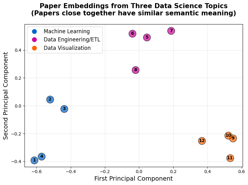
• The Machine Learning cluster (blue, papers 1-4) dominates the lower-left side of the plot. These four points sit close together because they all discuss neural networks, training, and model optimization. Look at papers 1 and 4. They're positioned very near each other despite one focusing on building networks from scratch and the other on transfer learning. The embedding model recognizes that they both use the core language of deep learning: layers, weights, training, and model architectures.
• The Data Engineering/ETL cluster (magenta, papers 5-8) occupies the upper portion of the plot. These papers share vocabulary around data quality, pipelines, and validation. Notice how papers 5, 6, and 7 form a tight grouping. They all discuss data quality issues using terms like "missing values," "validation," and "cleaning." Paper 8 (about Airflow) sits slightly apart from the others, which makes sense: while it's definitely about data engineering, it focuses more on workflow orchestration than data quality, giving it a slightly different semantic fingerprint.
• The Data Visualization cluster (orange, papers 9-12) is gathered on the lower-right side. These four papers are packed close together because they all use visualization-specific vocabulary: "charts," "dashboards," "colors," and "interactive elements." The tight clustering here shows just how distinct visualization terminology is from both ML and data engineering language.

What's remarkable is the clear separation between all three clusters. The distance between the ML papers on the left and the visualization papers on the right tells us that these topics use fundamentally different vocabularies. There's minimal semantic overlap between "neural networks" and "dashboards," so they end up far apart in the embedding space.

How the Model Learned to Understand Meaning

The all-MiniLM-L6-v2 embedding model was trained on millions of text pairs, learning which words tend to appear together. When it sees a tutorial full of words like "layers," "training," and "optimization," it produces an embedding vector that's mathematically similar to other texts with that same vocabulary pattern. The clustering emerges naturally from those learned associations.

Why This Matters for Your Work as an AI Engineer

Embeddings are foundational to the modern AI systems you'll build as an AI Engineer. Let's look at how embeddings enable the core technologies you'll work with:

1. Building Intelligent Search Systems

   Traditional keyword search has a fundamental limitation: it can only find exact matches. If a user searches for "handling null values," they won't find documents about "missing data strategies" or "imputation techniques," even though these are exactly what they need. Embeddings solve this by understanding semantic similarity. When you embed both the search query and your documents, you can find relevant content based on meaning rather than word matching. The result is a search system that actually understands what you're looking for.

2. Working with Vector Databases

   Vector databases are specialized databases that are built to store and query embeddings efficiently. Instead of SQL queries that match exact values, vector databases let you ask "find me all documents similar to this one" and get results ranked by semantic similarity. They're optimized for the mathematical operations that embeddings require, like calculating distances between high-dimensional vectors, which makes them essential infrastructure for AI applications. Modern systems often use hybrid search approaches that combine semantic similarity with traditional keyword matching to get the best of both worlds.

3. Implementing Retrieval-Augmented Generation (RAG)

   RAG systems are one of the most powerful patterns in modern AI engineering. Here's how they work: you embed a large collection of documents (like company documentation, research papers, or knowledge bases). When a user asks a question, you embed their question and use that embedding to find the most relevant documents from your collection. Then you pass those documents to a language model, which generates an informed answer grounded in your specific data. Embeddings make the retrieval step possible because they're how the system knows which documents are relevant to the question.

4. Creating AI Agents with Long-Term Memory

   AI agents that can remember past interactions and learn from experience need a way to store and retrieve relevant memories. Embeddings enable this. When an agent has a conversation or completes a task, you can embed the key information and store it in a vector database. Later, when the agent encounters a similar situation, it can retrieve relevant past experiences by finding embeddings close to the current context. This gives agents the ability to learn from history and make better decisions over time. In practice, long-term agent memory often uses similarity thresholds and time-weighted retrieval to prevent irrelevant or outdated information from being recalled.

These four applications (search, vector databases, RAG, and AI agents) are foundational tools for any aspiring AI Engineer's toolkit. Each builds on embeddings as a core technology. Understanding how embeddings capture semantic meaning is the first step toward building production-ready AI systems.

Advanced Topics to Explore

As you continue learning about embeddings, you'll encounter several advanced techniques that are widely used in production systems:

• Multimodal Embeddings allow you to embed different types of content (text, images, audio) into the same embedding space. This enables powerful cross-modal search capabilities, like finding images based on text descriptions or vice versa. Models like CLIP demonstrate how effective this approach can be.
• Instruction-Tuned Embeddings are models fine-tuned to better understand specific types of queries or instructions. These specialized models often outperform general-purpose embeddings for domain-specific tasks like legal document search or medical literature retrieval.
• Quantization reduces the precision of embedding values (from 32-bit floats to 8-bit integers, for example), which can dramatically reduce storage requirements and speed up similarity calculations with minimal impact on search quality. This becomes crucial when working with millions of embeddings.
• Dimension Truncation takes advantage of the fact that the most important information in embeddings is often concentrated in the first dimensions. By keeping only the first 256 dimensions of a 768-dimensional embedding, you can achieve significant efficiency gains while preserving most of the semantic information.

These techniques become increasingly important as you scale from prototype to production systems handling real-world data volumes.

Building Toward Production Systems

You've now learned the following core foundational embedding concepts:

• Embeddings convert text into numerical vectors that capture meaning
• Similar content produces similar vectors
• These relationships can be visualized to understand how the model organizes information

But we've only worked with 12 handwritten paper abstracts. This is perfect for getting the core concept, but real applications need to handle hundreds or thousands of documents.

In the next tutorial, we'll scale up dramatically. You'll learn how to collect documents programmatically using APIs, generate embeddings at scale, and make strategic decisions about different embedding approaches.

You'll also face the practical challenges that come with real data: rate limits on APIs, processing time for large datasets, the tradeoff between embedding quality and speed, and how to handle edge cases like empty documents or very long texts. These considerations separate a learning exercise from a production system.

By the end of the next tutorial, you'll be equipped to build an embedding system that handles real-world data at scale. That foundation will prepare you for our final embeddings tutorial, where we'll implement similarity search and build a complete semantic search engine.

Next Steps

For now, experiment with the code above:

• Try replacing one of the paper abstracts with content from your own learning.
  • Where does it appear on the visualization?
  • Does it cluster with one of our three topics, or does it land somewhere in between?
• Add a paper abstract that bridges two topics, like "Using Machine Learning to Optimize ETL Pipelines."
  • Does it position itself between the ML and data engineering clusters?
  • What does this tell you about how embeddings handle multi-topic content?
• Try changing the embedding model to see how it affects the visualization.
  • Models like all-mpnet-base-v2 produce different dimensional embeddings.
  • Do the clusters become tighter or more spread out?
• Experiment with adding a completely unrelated abstract, like a cooking recipe or news article.
  • Where does it land relative to our three data science clusters?
  • How far away is it from the nearest cluster?

This hands-on exploration and experimentation will deepen your intuition about how embeddings work.

Ready to scale things up? In the next tutorial, we'll work with real arXiv data and build an embedding system that can handle thousands of papers. See you there!

Key Takeaways:

• Embeddings convert text into numerical vectors that capture semantic meaning
• Similar meanings produce similar vectors, enabling mathematical comparison of concepts
• Papers from different topics cluster separately because they use distinct vocabulary
• Dimensionality reduction (like PCA) helps visualize high-dimensional embeddings in 2D
• Embeddings power modern AI systems, including semantic search, vector databases, RAG, and AI agents