Decision Trees in Machine Learning (Build One from Scratch)
Decision Trees represent one of the most popular machine learning algorithms. Here, we'll briefly explore their logic, internal structure, and even how to create one with a few lines of code.
In this article, we'll learn about the key characteristics of Decision Trees. There are different algorithms to generate them, such as ID3, C4.5 and CART. In our case, we'll be use CART, which is the algorithm used by one of the most popular Machine Learning libraries in Python: scikit-learn.
We'll also use this library to build and visualize a Decision Tree. This article assumes that you have at least a basic or intermediate coding knowledge using the Python language.

Structure and Components of Decision Trees
Before starting, let's get to know you a bit more and see if Dataquest can provide what you're looking for. Please answer the following questions with a "yes" or "no":
- Are you interested in learning Data Science?
- Do you prefer to learn online?
- Do you prefer to learn by doing?
- Are you interested in building a portfolio with Data Science projects?
If you answered "yes" to all these questions, then this is excellent news, because here at Dataquest, we share the same philosophy! But even if you answered "no", there is still some great news, as you inadvertently used logic to build a Decision Tree!
If we translate this process to Python code, such logic could be understood as the sum of different if/else statements, which can be represented like this:
print("Are you interested in learning Data Science?")
    if True:
        print("Do you prefer to learn online?")
            if True:
                print("Do you prefer to learn by doing?")
                    if True:
                        print("Are you interested in building a portfolio with Data Science projects?")
                            if True:
                                print("Dataquest can give you what you want!")
                            if False:
                                print("Would you give it a chance?")
                    if False:
                        print("Would you give it a chance?")
            if False:
                print("Would you give it a chance?")
    if False:
        print("Would you give it a chance?")`
However, while this logic would be familiar to people with at least some basic understanding of Python (and coding in general), the same can't be said for people with no coding experience at all, and this is one of the biggest advantages of Decision Trees: we can present them graphically, in a way that can be understood by general audiences, after giving them some specific instructions about how to interpret them.
Let's present the previous logic with a proper Decision Tree graphic, for which we'll then explain the components and general structure. This is how it would look:
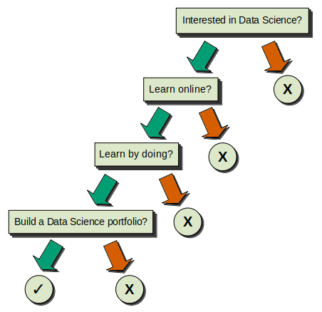
Now that the tree is properly presented, we can continue exploring its structure. Let's focus on the components we see:
1) We have four squares with the questions inside, and five circles — four of these are negative (X) and one is positive (✓). All of these are called Nodes.

- The squared node at the top is called the Root Node, because it doesn't originate from any other node, and because it's also the most important node. When we build our Decision Trees, this is the node with the most predictive power. Notice that it's called root in reference to a tree's root, so that's why we used an inverted tree image at the beginning of this article: it means that the Decision Trees are interpreted as inverted trees!

- The rest of the squared nodes are called Internal Nodes, and their key characteristic is that they always originate from a previous node (they are the Child Nodes of the previous node). At the same time, they also generate subsequent nodes (they are the Parent Nodes of those subsequent nodes).

- Following the logic of the inverted tree, we'll always end in the circular nodes, which are called Terminal Nodes or--most commonly--Leaves. Since they're final, they're also always Child Nodes, as they can't never generate more nodes. These Leaves are critical, because they inform us of the result of the choices we made during the process.
2) For every Root Node and Internal Node, there are two arrows that emerge from them, one green and one red. In addition to the Root Node, we have three Internal Nodes in this example, so we get a total of eight arrows. These arrows are called the Branches.

-
The green arrows represent the path we follow if the answer to the condition/question equates to True. So, for example, if we have the question "Do you like to learn by doing?" and we answer "yes", then it's True, and we continue to the left node below.
-
The red arrows represent the opposite; all the answers to the condition/question that equate to False continue to the right node below.
It's important that we remember this, as it's universal to Decision Trees: Left == True. Right == False.
Now that we've described every component of the Decision Tree, we can answer the four questions again to see how our decisions would flow across the graphic.
One of the questions was "Do you like to learn by doing?" Obviously, as we expressed before, we live by that principle, so in the next section we'll explore how to create a Decision Tree from scratch, by using a specific dataset and the powerful library scikit-learn!
Introducing the Dataset
The dataset we'll use on this occasion is "Estimation of obesity levels based on eating habits and physical condition", which can be found on the UCI Machine Learning Repository site, which includes information about obesity cases in Mexico, Peru and Colombia.
Let's load it and check the first observations to get a general idea of the information:
import pandas as pd

df = pd.read_csv("ObesityDataSet_raw_and_data_sinthetic.csv")
df.iloc[:10, :11]| Gender | Age | Height | Weight | family_history_with_overweight | FAVC | FCVC | NCP | CAEC | SMOKE | CH2O | SCC | FAF | TUE | |
|---|---|---|---|---|---|---|---|---|---|---|---|---|---|---|
| 0 | Female | 21.0 | 1.62 | 64.0 | yes | no | 2.0 | 3.0 | Sometimes | no | 2.0 | no | 0.0 | 1.0 |
| 1 | Female | 21.0 | 1.52 | 56.0 | yes | no | 3.0 | 3.0 | Sometimes | yes | 3.0 | yes | 3.0 | 0.0 |
| 2 | Male | 23.0 | 1.80 | 77.0 | yes | no | 2.0 | 3.0 | Sometimes | no | 2.0 | no | 2.0 | 1.0 |
| 3 | Male | 27.0 | 1.80 | 87.0 | no | no | 3.0 | 3.0 | Sometimes | no | 2.0 | no | 2.0 | 0.0 |
| 4 | Male | 22.0 | 1.78 | 89.8 | no | no | 2.0 | 1.0 | Sometimes | no | 2.0 | no | 0.0 | 0.0 |
| 5 | Male | 29.0 | 1.62 | 53.0 | no | yes | 2.0 | 3.0 | Sometimes | no | 2.0 | no | 0.0 | 0.0 |
| 6 | Female | 23.0 | 1.50 | 55.0 | yes | yes | 3.0 | 3.0 | Sometimes | no | 2.0 | no | 1.0 | 0.0 |
| 7 | Male | 22.0 | 1.64 | 53.0 | no | no | 2.0 | 3.0 | Sometimes | no | 2.0 | no | 3.0 | 0.0 |
| 8 | Male | 24.0 | 1.78 | 64.0 | yes | yes | 3.0 | 3.0 | Sometimes | no | 2.0 | no | 1.0 | 1.0 |
| 9 | Male | 22.0 | 1.72 | 68.0 | yes | yes | 2.0 | 3.0 | Sometimes | no | 2.0 | no | 1.0 | 1.0 |
df.iloc[:10, 11:]| CALC | MTRANS | NObeyesdad | |
|---|---|---|---|
| 0 | no | Public_Transportation | Normal_Weight |
| 1 | Sometimes | Public_Transportation | Normal_Weight |
| 2 | Frequently | Public_Transportation | Normal_Weight |
| 3 | Frequently | Walking | Overweight_Level_I |
| 4 | Sometimes | Public_Transportation | Overweight_Level_II |
| 5 | Sometimes | Automobile | Normal_Weight |
| 6 | Sometimes | Motorbike | Normal_Weight |
| 7 | Sometimes | Public_Transportation | Normal_Weight |
| 8 | Frequently | Public_Transportation | Normal_Weight |
| 9 | no | Public_Transportation | Normal_Weight |
We can also explore the different columns:
df.info()
RangeIndex: 2111 entries, 0 to 2110
Data columns (total 17 columns):
 #   Column                          Non-Null Count  Dtype
---  ------                          --------------  -----
 0   Gender                          2111 non-null   object
 1   Age                             2111 non-null   float64
 2   Height                          2111 non-null   float64
 3   Weight                          2111 non-null   float64
 4   family_history_with_overweight  2111 non-null   object
 5   FAVC                            2111 non-null   object
 6   FCVC                            2111 non-null   float64
 7   NCP                             2111 non-null   float64
 8   CAEC                            2111 non-null   object
 9   SMOKE                           2111 non-null   object
 10  CH2O                            2111 non-null   float64
 11  SCC                             2111 non-null   object
 12  FAF                             2111 non-null   float64
 13  TUE                             2111 non-null   float64
 14  CALC                            2111 non-null   object
 15  MTRANS                          2111 non-null   object
 16  NObeyesdad                      2111 non-null   object
dtypes: float64(8), object(9)
memory usage: 280.5+ KB
We can see that the dataset contains 17 columns and 2111 observations. While some of the column names are self-explanatory, like Gender, Age, Height, Weight, family_history_with_overweight (binary: yes/no) and SMOKE (binary: yes/no), there are other column names which are acronyms, so we need to clarify what information they contain:
-
FAVC: Frequent consumption of high caloric food (binary: yes/no).
-
FCVC: Frequency of consumption of vegetables (numeric)
-
NCP: Number of main meals (numeric)
-
CAEC: Consumption of food between meals (ordinal: no/sometimes/frequently/always)
-
CH20: Consumption of water daily (numeric)
-
CALC: Consumption of alcohol (ordinal: no/sometimes/frequently/always)
-
SCC: Calories consumption monitoring (binary: yes/no)
-
FAF: Physical activity frequency (numeric)
-
TUE: Time using technology devices (numeric)
-
MTRANS: Transportation used (categorical: public_transportation, automobile, walking, motorbike, bike)
As for the target column, it's NObeyesdad (obesity level), and the following are the possible class values, along with the observation count for each one:
df["NObeyesdad"].value_counts()Obesity_Type_I 351
Obesity_Type_III 324
Obesity_Type_II 297
Overweight_Level_I 290
Overweight_Level_II 290
Normal_Weight 287
Insufficient_Weight 272
Name: NObeyesdad, dtype: int64Since scikit-learn requires us to use only numerical data, we'll need to preprocess the dataset to transform the feature columns to numbers.
Preparing the Dataset
As expressed, in this section, we’ll perform data cleaning on the dataset to prepare it for building the machine learning model in the next section.
We’ll frequently use .value_counts() from the pandas library for every column, which returns the counts of all distinct values from each specific column.
In this case, from our 2111 total observations, we see that for the "Gender" column we have 1068 males and 1043 females.
# "GENDER" COLUMN

df["Gender"].value_counts()
Male 1068
Female 1043
Name: Gender, dtype: int64Since the column is binary (it only includes two possible values), we can transform it to numerical values by making it boolean.
We do this by taking any gender we want (in this case, we chose female) and replacing every observation with 0 if it equates to False (that is, if it's a male), and 1 if the observation equates to True (the observation is about a female).
Finally, we'll rename the column female to reflect this change and avoid confusion in the future:
df["Gender"].replace({"Male": 0, "Female": 1}, inplace = True)

df.rename(columns = {"Gender": "female"}, inplace = True)
Just to be cautious, we'll double check how the data transformation went by using .value_counts() again. Note how we're using the new column name now:
# Double Check

df["female"].value_counts()
0 1068
1 1043
Name: female, dtype: int64We can confirm that the transformation was successful. We have 1068 False/0 observations, which represent males, and 1043 True/1 observations, which represent females. This matches the original value counts before the transformation.
Let's apply the same steps to the following column:
# "FAMILY HISTORY WITH OVERWEIGHT" COLUMN

df["family_history_with_overweight"].value_counts()
yes 1726
no 385
Name: family_history_with_overweight, dtype: int64df["family_history_with_overweight"].replace({"no": 0, "yes": 1}, inplace = True)
df.rename(columns = {"family_history_with_overweight": "family_history_overweight"}, inplace = True)# Double Check
df["family_history_overweight"].value_counts()1 1726
0 385
Name: family_history_overweight, dtype: int64We'll continue performing the same steps, but for this case, we don't need to rename the column:
# "FREQUENT CONSUMPTION OF HIGH CALORIC FOOD" COLUMN

df["FAVC"].value_counts()
yes 1866
no 245
Name: FAVC, dtype: int64df["FAVC"].replace({"no": 0, "yes": 1}, inplace = True)# Double Check
df["FAVC"].value_counts()1 1866
0 245
Name: FAVC, dtype: int64The following column is a more complex case, because not only do we have more than two unique values (in other words, it's no longer binary), but the different values are related to each other with a hierarchy (in this case, frequency):
No > Sometimes > Frequently > Always
This is a clear example of an ordinal column.
# "CONSUMPTION OF FOOD BETWEEN MEALS" COLUMN

df["CAEC"].value_counts()
Sometimes 1765
Frequently 242
Always 53
no 51
Name: CAEC, dtype: int64In this situation, when transforming the data to numeric values, we can reflect that hierarchy by using consecutive numbers, starting with the lowest value as 0, and ending with the highest value having the highest number.
No == 0
Sometimes == 1
Frequently == 2
Always == 3
This is an extremely simplified explanation, and we cover this subject in more detail in the Decision Trees course.
from sklearn.preprocessing import OrdinalEncoder

ordinal_caec = [["no", "Sometimes", "Frequently", "Always"]]

df["CAEC"] = OrdinalEncoder(categories = ordinal_caec).fit_transform(df[["CAEC"]])
We can confirm that the hierarchy was preserved during the transformation to numeric values:
# Double Check

df["CAEC"].value_counts()
1.0 1765
2.0 242
3.0 53
0.0 51
Name: CAEC, dtype: int64The following columns are binary, so there isn't much to discuss, for the moment. We'll simply apply the same steps from above:
# "SMOKE" COLUMN

df["SMOKE"].value_counts()
no 2067
yes 44
Name: SMOKE, dtype: int64df["SMOKE"].replace({"no": 0, "yes": 1}, inplace = True)# Double Check
df["SMOKE"].value_counts()0 2067
1 44
Name: SMOKE, dtype: int64# "CALORIES CONSUMPTION MONITORING" COLUMN
df["SCC"].value_counts()no 2015
yes 96
Name: SCC, dtype: int64df["SCC"].replace({"no": 0, "yes": 1}, inplace = True)# Double Check
df["SCC"].value_counts()0 2015
1 96
Name: SCC, dtype: int64The following column is also ordinal, and since it shares the exact same hierarchy (frequency) as the previous one, we'll perform the same steps as before:
# "CONSUMPTION OF ALCOHOL" COLUMN

df["CALC"].value_counts()
Sometimes 1401
no 639
Frequently 70
Always 1
Name: CALC, dtype: int64from sklearn.preprocessing import OrdinalEncoder
ordinal_calc = [["no", "Sometimes", "Frequently", "Always"]]
df["CALC"] = OrdinalEncoder(categories = ordinal_calc).fit_transform(df[["CALC"]])# Double Check
df["CALC"].value_counts()1.0 1401
0.0 639
2.0 70
3.0 1
Name: CALC, dtype: int64In this last column, we have another special case: while we have more than two distinct values, we don’t have a hierarchy here. The distinct values represent different options that aren't related to each other via a hierarchy. They're independent in this sense; therefore, the column is categorical.
# "TRANSPORTATION USED" COLUMN

df["MTRANS"].value_counts()
Public_Transportation 1580
Automobile 457
Walking 56
Motorbike 11
Bike 7
Name: MTRANS, dtype: int64Since we can't assign a different number to each value, because this would create an unintentional hierarchy, what we have to do in this case is create a new column for every single value; then we'll use the boolean approach: if the observation mentions a certain transportation, the corresponding column that refers to that transportation type will have "1", and the rest of the columns will have "0". We'll see how this looks when we double check.
This is the necessary code to perform the operation, which, due to its complexity, will be dissected in detail in the Decision Trees course.
from sklearn.preprocessing import OneHotEncoder
from sklearn.compose import make_column_transformer

col_trans = make_column_transformer((OneHotEncoder(), ["MTRANS"]),
                                    remainder = "passthrough",
                                    verbose_feature_names_out = False)

onehot_df = col_trans.fit_transform(df)

df = pd.DataFrame(onehot_df, columns = col_trans.get_feature_names_out())
It's important to note that during this transformation, the column that includes all the different values together ("MTRANS") will be erased, as it won't be needed anymore.
Let's check the transformation. Instead of "MTRANS", we now have five different columns, each one representing a possible value for "MTRANS": MTRANS_Automobile, MTRANS_Bike, MTRANS_Motorbike, MTRANS_Public_Transportation and MTRANS_Walking.
# Double Check

df.iloc[:10, :9]| MTRANS_Automobile | MTRANS_Bike | MTRANS_Motorbike | MTRANS_Public_Transportation | MTRANS_Walking | female | Age | Height | Weight | |
|---|---|---|---|---|---|---|---|---|---|
| 0 | 0.0 | 0.0 | 0.0 | 1.0 | 0.0 | 1 | 21.0 | 1.62 | 64.0 |
| 1 | 0.0 | 0.0 | 0.0 | 1.0 | 0.0 | 1 | 21.0 | 1.52 | 56.0 |
| 2 | 0.0 | 0.0 | 0.0 | 1.0 | 0.0 | 0 | 23.0 | 1.8 | 77.0 |
| 3 | 0.0 | 0.0 | 0.0 | 0.0 | 1.0 | 0 | 27.0 | 1.8 | 87.0 |
| 4 | 0.0 | 0.0 | 0.0 | 1.0 | 0.0 | 0 | 22.0 | 1.78 | 89.8 |
| 5 | 1.0 | 0.0 | 0.0 | 0.0 | 0.0 | 0 | 29.0 | 1.62 | 53.0 |
| 6 | 0.0 | 0.0 | 1.0 | 0.0 | 0.0 | 1 | 23.0 | 1.5 | 55.0 |
| 7 | 0.0 | 0.0 | 0.0 | 1.0 | 0.0 | 0 | 22.0 | 1.64 | 53.0 |
| 8 | 0.0 | 0.0 | 0.0 | 1.0 | 0.0 | 0 | 24.0 | 1.78 | 64.0 |
| 9 | 0.0 | 0.0 | 0.0 | 1.0 | 0.0 | 0 | 22.0 | 1.72 | 68.0 |
For the very first observation, for example, since that person used public transportation, the corresponding MTRANS_Public_Transportation column was marked with 1 ("True"), and the other four columns were marked with 0 ("False").
df.iloc[:10, 9:]| family_history_overweight | FAVC | FCVC | NCP | CAEC | SMOKE | CH2O | SCC | FAF | TUE | CALC | NObeyesdad | |
|---|---|---|---|---|---|---|---|---|---|---|---|---|
| 0 | 1 | 0 | 2.0 | 3.0 | 1.0 | 0 | 2.0 | 0 | 0.0 | 1.0 | 0.0 | Normal_Weight |
| 1 | 1 | 0 | 3.0 | 3.0 | 1.0 | 1 | 3.0 | 1 | 3.0 | 0.0 | 1.0 | Normal_Weight |
| 2 | 1 | 0 | 2.0 | 3.0 | 1.0 | 0 | 2.0 | 0 | 2.0 | 1.0 | 2.0 | Normal_Weight |
| 3 | 0 | 0 | 3.0 | 3.0 | 1.0 | 0 | 2.0 | 0 | 2.0 | 0.0 | 2.0 | Overweight_Level_I |
| 4 | 0 | 0 | 2.0 | 1.0 | 1.0 | 0 | 2.0 | 0 | 0.0 | 0.0 | 1.0 | Overweight_Level_II |
| 5 | 0 | 1 | 2.0 | 3.0 | 1.0 | 0 | 2.0 | 0 | 0.0 | 0.0 | 1.0 | Normal_Weight |
| 6 | 1 | 1 | 3.0 | 3.0 | 1.0 | 0 | 2.0 | 0 | 1.0 | 0.0 | 1.0 | Normal_Weight |
| 7 | 0 | 0 | 2.0 | 3.0 | 1.0 | 0 | 2.0 | 0 | 3.0 | 0.0 | 1.0 | Normal_Weight |
| 8 | 1 | 1 | 3.0 | 3.0 | 1.0 | 0 | 2.0 | 0 | 1.0 | 1.0 | 2.0 | Normal_Weight |
| 9 | 1 | 1 | 2.0 | 3.0 | 1.0 | 0 | 2.0 | 0 | 1.0 | 1.0 | 0.0 | Normal_Weight |
Finally, we don't need to transform the target column "NObeyesdad" to numeric, since it features the possible classes that the Decision Tree will try to predict.
Building Our Own Decision Tree
scikit-learn is a pretty standardized library, which means that it allows us to instantiate and train our Machine Learning models in a few lines of code. This will apply to Decision Trees as well.
As a reminder, scikit-learn uses the CART algorithm, which stands for Classification And Regression Trees; therefore, we can build Decision Trees to predict both classification and regression problems!
As a quick recap, when we say classification, we're referring to predicting a categorical label, which can be binary (e.g., positive/negative, on/off, true/false etc.) or a limited number of categories (e.g., colors, seasons, months, etc.), whereas regression refers to predicting numerical quantities (e.g., price, age, distance, etc.).
In this case, we'll stick with a Classification Tree, as the dataset includes classes/categories in its target column.
df["NObeyesdad"].unique()array(['Normal_Weight', 'Overweight_Level_I', 'Overweight_Level_II',
'Obesity_Type_I', 'Insufficient_Weight', 'Obesity_Type_II',
'Obesity_Type_III'], dtype=object)The first step of scikit-learn to create a Machine Learning model is to divide the dataset between the feature columns (X) and the target column (y). Note that we remove the "NObeyesdad" column from X, given that it contains the target values.
X = df.drop(["NObeyesdad"], axis = 1)
y = df["NObeyesdad"]
Now we'll import the Decision Tree model for classification, along with train_test_split.
from sklearn.tree import DecisionTreeClassifier
from sklearn.model_selection import train_test_split
train_test_split is a tool that allows us to divide the dataset in four sections, which will be stored in distinct variables: X_train and y_train contain the observations to train the model, while X_test and y_test contain the observations to test the model's accuracy.
The test_size parameter sets the percentage of observations from the dataset that will be used for testing purposes. In this case, 0.2 is a commonly-used proportion that translates to 20% of the total number.
As for random_state, it's simply a number that ensures reproducibility of results, and for that reason you'll often see it as a parameter for different functions.
X_train, X_test, y_train, y_test = train_test_split(X, y, test_size = 0.2, random_state = 14)And now, this is the moment our Decision Tree is born!
One important thing to consider: while it may be common in other machine learning algorithms to not include any parameters at all, in the case of Decision Trees we're required to set a value for the max_depth parameter.
This parameter determines the depth of the Tree. In other words, it prunes several Internal Nodes in order to avoid an undesirable phenomena called overfitting, which happens when the Tree adapts so closely to the dataset that it then becomes unable to make predictions on unseen data.
In this case, a max_depth = 4 indicates that we'll limit the Tree to four levels: the root node, two intermediate levels, and the final level, where the Leaves are.
tree = DecisionTreeClassifier(max_depth = 4, random_state = 14)Excellent! Now that the Tree has been brought into existence, we'll train it using the training data we stored in X_train and y_train:
tree.fit(X_train, y_train)Now we need to know if the generated Tree is good enough, in terms of accuracy (how well it predicts unseen data). We can quickly determine this by using the score method, which Decision Trees share with other Machine Learning algorithms.
tree.score(X_test, y_test)0.7848699763593381Notice the low number of lines of code required to generate and evaluate the Decision Tree: just eight! scikit-learn definitely makes this process a very straightforward one!
Regarding the score: while a perfect value is 1.0, in real life it’s impossible to achieve it (or even worse: if we actually achieve it, it means that our machine learning model is overfitting!). Although there isn’t a defined metric, and every data situation is different, in general we can be confident that an accuracy score higher than 0.7 indicates that the model is pretty good, which is the result we got here!
But we also have to consider the subject we're dealing with: since it's health related, "pretty good" has to be the starting point of further optimizations, as we need to ensure the highest possible accuracy (i.e. around 0.95, ideally), given that misclassifying an observation could end up having truly adverse consequences in real life. We need to conduct ourselves with the utmost prudence in these kinds of scenarios.
In the following section, we'll explore the final stage of our small journey, which is visualizing the Decision Tree and gaining insights from it!
Visualizing the Tree
As always, scikit-learn ensures that our Machine Learning tasks become direct and standardized, and visualizing the Decision Trees is no exception!
For this case, we'll use the plot_tree tool, but we'll also use the additional library matplotlib, related to data visualization. This will allow us to adjust the image size by using the figure method.
Apart from that initial code, the following are the parameters that we're required to write in order to customize the Tree visualization:
-
decision_tree: The variable where the Decision Tree was instantiated.
-
feature_names: The names of the feature columns, which can quickly be accessed with
X.columns. -
class_names: The name of the classes/categories in the target column, which can be quickly accessed with
tree.classes_(if your Decision Tree was created with another variable name, you would replace the variable name accordingly). -
filled: If set to True, this parameter assigns a distinct color to every class, and every Node will be painted with the color of the dominant class. In addition, the color may be more or less intense, contingent to how dominant the class is in that Node.
-
fontsize: Size of the font inside the nodes.
-
impurity: (We set this to False to omit one specific piece of information; since this is an introductory article, explaining this value would greatly extend the article's length. Also, we would need to delve into more complex explanations).
An important clarification regarding the _ variable: while it's possible to use plot_tree directly, without assigning the function to a variable, this would've created verbose text before the visualization, something we prefer to avoid to ensure a cleaner display.
Once we finish customizing these parameters, we formally plot the Decision Tree with plt.show().
from sklearn.tree import plot_tree
import matplotlib.pyplot as plt

plt.figure(figsize = [24.0, 12.0])

_ = plot_tree(
          decision_tree = tree,
          feature_names = X.columns,
          class_names =  tree.classes_,
          impurity = False,
          filled = True,
          fontsize = 11)

plt.show()
The information displayed by every node is definitely more comprehensive than the theoretical diagram we used at the beginning of the article, so let's dissect what we see here to clarify any confusion:
- The uppermost line in every node represents the condition used to split the decision path. Since
scikit-learnonly works with numerical information, this condition will always be translated to a threshold. In other words, instead of having a question, like "Do you prefer to learn by doing?", we'll always have a column name and a comparison with a specific number.
For example, if we have Weight <= 76.063, then all the observations where Weight is lower or equal to 76.063 will be evaluated to True, so we would continue to the left child node. On the opposite side, all the observations whose value is higher than 76.063 would evaluate to False, and we would continue to the right child node (i.e. 78 <= 76.063 evaluates to False, as 78 is a higher number than 76.063).
Remember: Left == True. Right == False!
- The samples field refers to the total number of observations classified under that Node after splitting the information.
In this sense, the "samples" field in the root node will always equal the total number of observations of the dataset. (Note that here we only have 1688 observations instead of 2111 because we isolated some observations for testing purposes!)

If we check the two nodes in the following level, we see that the left child node has 1115 observations that equate to True, while the right child node has 573 observations that equate to False. If we sum them (1115 + 573) we'll get 1688, the samples value from the root node.
-
The value field filters the number from samples to indicate the number of observations per target class. For instance, if we focus on the root node, and we sum all the numbers from the value field, we'll get the samples number. This rules applies to all nodes.
To determine to which target class every number belongs, we have to match the order with the one in the
classes_attribute:
tree.classes_array(['Insufficient_Weight', 'Normal_Weight', 'Obesity_Type_I',
'Obesity_Type_II', 'Obesity_Type_III', 'Overweight_Level_I',
'Overweight_Level_II'], dtype=object)As an example, if we have the values [215, 227, 287, 246, 236, 234, 243] from the root node, we would match them like this:
values = [215, 227, 287, 246, 236, 234, 243]
classes = tree.classes_
list(zip(classes, values))
[('Insufficient_Weight', 215),
('Normal_Weight', 227),
('Obesity_Type_I', 287),
('Obesity_Type_II', 246),
('Obesity_Type_III', 236),
('Overweight_Level_I', 234),
('Overweight_Level_II', 243)]-
Finally, we have the class field, which indicates the dominant target class in every node.
Note that, as we expressed earlier,
scikit-learnassigns a specific color to every target class, so, for instance, the Insufficient Weight class has brown-colored nodes with different shades, depending on how much dominance that class has in each node.
For example, for the middle left node Height <= 1.66, although the class has 209 observations there (higher than the other brown nodes), because the following class (Normal Weight) has a high number of observations as well (114), Insufficient Weight isn't as dominant there, and it gets a lighter color, despite having more observations of that target class compared with the other brown nodes.
On the other hand, and most importantly, if we want to predict the result of our own observations, we need to reach a Leaf Node and read the class there to learn to which target class our observation would belong.


Now that we've seen every component of the plotted Decision Tree, we're going to use it to predict the weight classification of these women:
1) Guadalupe, who has a Weight of 75 and a Height of 1.80

(Image generated at This Person Does Not Exist.)

First we have the root node, Weight <= 99.536. Guadalupe weights 75, so the threshold condition evaluates to True, and we descend to the left child node.

There we have a threshold Weight <= 60.059, so 75 <= 60.059 evaluates to False, and in this case we descend to the right child node.

In this third node we have Weight <= 76.063, so 75 <= 76.063 evaluates to True and we descend to the left child node.

The threshold of the fourth node is Height <= 1.735, so 1.80 <= 1.735 evaluates to False and we reach the right child node, which is the Leaf, and the target class is Normal Weight.

Therefore, Guadalupe has a healthy weight!
2) Camila, whose Weight is 111

(Image generated at This Person Does Not Exist.)
First we have the root node, Weight <= 99.536. Camila weighs 111, so the threshold condition evaluates to False and we descend to the right child node.

In this second node, the threshold says female <= 0.5. Considering that when we preprocessed the data we altered the Gender column to make it numeric, now instead of male/female the column was renamed as female, and the value is 0 if it's False (male) and 1 if it's True (female).
So, because of this, female evaluates to 1, so 1 <= 0.5 evaluates to False and we descend to the right child node, which is the Leaf, and the target class is Obesity_Type_III:

So Camila unfortunately doesn't have an optimal weight.
Conclusion
Decision Trees are one of the most popular Machine Learning algorithms, and this is because they're relatively easier to understand compared to other algorithms, due to the way we can build graphical representations of their insights.
In this blog post, we covered the following:
-
The overall structure of Decision Trees.
-
How to interpret Decision Trees.
-
How to create our own Decision Trees with
scikit-learn. -
How to visualize our own Decision Trees.
However, this is just an introductory article; these and other aspects are covered in-depth in our dedicated course for Decision Trees. Besides the points above, here are some of the other subjects explored in detail there:
-
How Decision Trees are generated under the surface.
-
Data preprocessing to train Decision Trees (including some useful
scikit-learntools that aren't widely known!) -
Creation of both Classification and Regression Trees.
-
Advantages and disadvantages of Decision Trees.
-
Evaluation of Decision Trees' efficiency, including cross-validated approaches.
-
Pruning and optimization of Decision Trees.
-
Ensemble techniques, including Random Forest and Extra Trees.
If you're interested in learning more, check out our Decision Tree and Random Forest Modeling in Python course.