Running and Managing Apache Airflow with Docker (Part I)

In the last tutorial, we explored what workflow orchestration is, why it matters, and how Apache Airflow structures, automates, and monitors complex data pipelines through DAGs, tasks, and the scheduler. We examined how orchestration transforms scattered scripts into a coordinated system that ensures reliability, observability, and scalability across modern data workflows.

In this two-part hands-on tutorial, we move from theory to practice. You’ll run Apache Airflow inside Docker, the most efficient and production-like way to deploy Airflow for development and testing. This containerized approach mirrors how Airflow operates in real-world environments, from on-premises teams to managed services like ECR and Cloud Composer.

In Part One, our focus goes beyond setup. You’ll learn how to work effectively with DAGs inside a Dockerized Airflow environment, writing, testing, visualizing, and managing them through the Web UI. You’ll use the TaskFlow API to build clean, Pythonic workflows and implement dynamic task mapping to run multiple processes in parallel. By the end of this part, you’ll have a fully functional Airflow environment running in Docker and a working DAG that extracts and transforms data automatically, the foundation of modern data engineering pipelines.

In Part Two, we’ll extend that foundation to handle data management and automation workflows. You’ll connect Airflow to a local MySQL database for data loading, manage credentials securely through the Admin panel and environment variables, and integrate Git with Git Sync to enable version control and continuous deployment. You’ll also see how CI/CD pipelines can automate DAG validation and deployment, ensuring your Airflow environment remains consistent and collaborative across development teams.

By the end of the series, you’ll not only understand how Airflow runs inside Docker but also how to design, orchestrate, and manage production-grade data pipelines the way data engineers do in real-world systems.

Why Use Docker for Airflow

While Airflow can be installed locally with pip install apache-airflow, this approach often leads to dependency conflicts, version mismatches, and complicated setups. Airflow depends on multiple services, an API server, scheduler, triggerer, metadata database, and dag-processors, all of which must communicate correctly. Installing and maintaining these manually on your local machine can be tedious and error-prone.

Docker eliminates these issues by packaging everything into lightweight, isolated containers. Each container runs a single Airflow component, but all work together seamlessly through Docker Compose. The result is a clean, reproducible environment that behaves consistently across operating systems.

In short:

• Local installation: works for testing but often breaks due to dependency conflicts or version mismatches.
• Cloud-managed services (like AWS ECS or Cloud Composer): excellent for production but not that much flexible for learning or prototyping.
• Docker setup: combines realism with simplicity, providing the same multi-service environment used in production without the overhead of manual configuration.

Docker setup is ideal for learning and development and closely mirrors production environments, but additional configuration is needed for a full production deployment

Prerequisites

Before you begin, ensure the following are installed and ready on your system:

1. Docker Desktop – Required to build and run Airflow containers.
2. A code editor – Visual Studio Code or similar, for writing and editing DAGs.
3. Python 3.10 or higher – Used for authoring Airflow DAGs and helper scripts.

Running Airflow Using Docker

Now that your environment is ready (Docker is open and running), let’s get Airflow running using Docker Compose.

This tool orchestrates all Airflow services, api-server, scheduler, triggerer, database, and workers — so they start and communicate properly.

Clone the Tutorial Repository

We’ve already prepared the starter files you’ll need for this tutorial on GitHub.

Begin by cloning the repository:

git clone [email protected]:dataquestio/tutorials.git

Then navigate to the Airflow tutorial folder:

cairflow-docker-tutorial

This is the directory where you’ll be working throughout the tutorial.

Inside, you’ll notice a structure similar to this:

airflow-docker-tutorial/
├── part-one/  
├── part-two/
├── docker-compose.yaml
└── README.md

• The part-one/ and part-two/ folders contain the complete reference files for both tutorials (Part One and Part Two).

  You don’t need to modify anything there, it’s only for comparison or review.

• The docker-compose.yaml file is your starting point and will evolve as the tutorial progresses.

Explore the Docker Compose File

Open the docker-compose.yaml file in your code editor.

This file defines all the Airflow components and how they interact inside Docker.

It includes:

• api-server – Airflow’s web user interface
• Scheduler – Parses and triggers DAGs
• Triggerer – Manages deferrable tasks efficiently
• Metadata database – Tracks DAG runs and task states
• Executors – Execute tasks

Each of these services runs in its own container, but together they form a single working Airflow environment.

You’ll be updating this file as you move through the tutorial to configure, extend, and manage your Airflow setup.

Create Required Folders

Airflow expects certain directories to exist before launching.

Create them inside the same directory as your docker-compose.yaml file:

mkdir -p ./dags ./logs ./plugins ./config

• dags/ – your workflow scripts
• logs/ – task execution logs
• plugins/ – custom hooks and operators
• config/ – optional configuration overrides (this will be auto-populated later when initializing the database)

Configure User Permissions

If you’re using Linux, set a user ID to prevent permission issues when Docker writes files locally:

echo -e "AIRFLOW_UID=$(id -u)" > .env

If you’re using macOS or Windows, manually create a .env file in the same directory with the following content:

AIRFLOW_UID=50000

This ensures consistent file ownership between your host system and the Docker containers.

Initialize the Metadata Database

Airflow keeps track of DAG runs, task states, and configurations in a metadata database.

Initialize it by running:

docker compose up airflow-init

Once initialization completes, you’ll see a message confirming that an admin user has been created with default credentials:

• Username: airflow
• Password: airflow

Start Airflow

Now start all Airflow services in the background:

docker compose up -d

Docker Compose will spin up the scheduler, API server, triggerer, database, and worker containers.

Step 6: Start Airflow

Now launch all the services in the background:

docker compose up -d

Docker Compose will start the scheduler, api-server, triggerer, database, and executor containers.

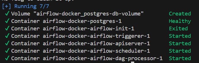
Make sure the triggerer, dag-processor, scheduler, and api-server are shown as started as above. If that is not the case, rebuild the Docker container, since the build process might have been interrupted. Otherwise, navigate to http://localhost:8080 to access the Airflow UI exposed by the api-server.

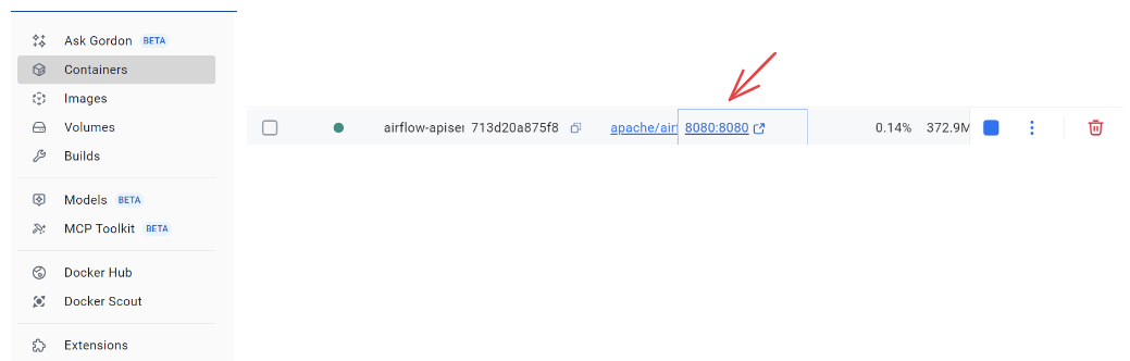
You can also access this through your Docker app, by navigating to containers:

Log in using the credentials above to accessh the Airflow Web UI.

• If the UI fails to load or some containers keep restarting, increase Docker’s memory allocation to at least 4 GB (8 GB recommended) in Docker Desktop → Settings → Resources.

Configuring the Airflow Project

Once Airflow is running and you visit http://localhost:8080, you’ll be seee Airflow Web UI.

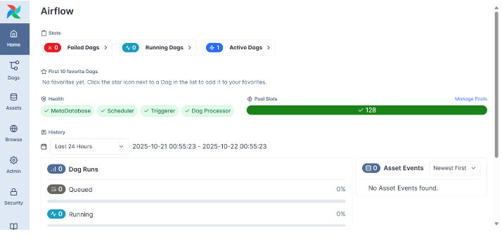
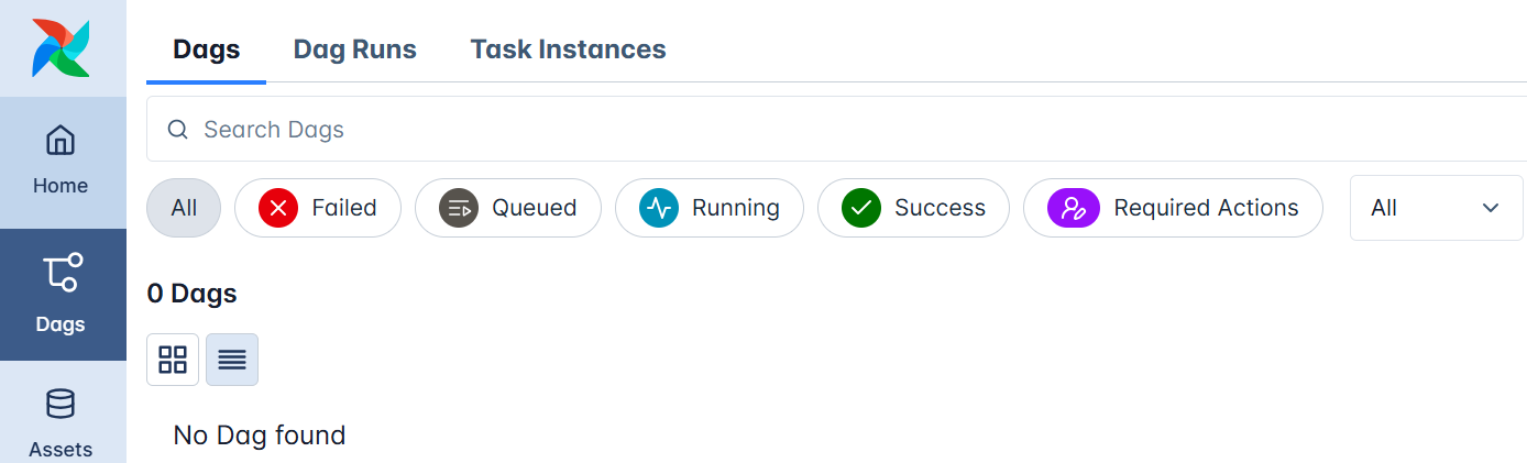
This is the command center for your workflows, where you can visualize DAGs, monitor task runs, and manage system configurations. When you navigate to Dags, you’ll see a dashboard that lists several example DAGs provided by the Airflow team. These are sample workflows meant to demonstrate different operators, sensors, and features.

However, for this tutorial, we’ll build our own clean environment, so we’ll remove these example DAGs and customize our setup to suit our project.

Before doing that, though, it’s important to understand the docker-compose.yaml file, since this is where your Airflow environment is actually defined.

Understanding the docker-compose.yaml File

The docker-compose.yaml file tells Docker how to build, connect, and run all the Airflow components as containers.

If you open it, you’ll see multiple sections that look like this:

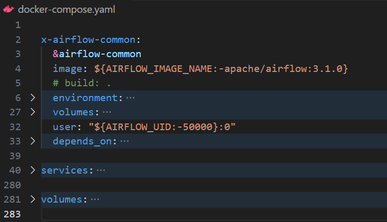
Let’s break this down briefly:

• x-airflow-common – This is the shared configuration block that all Airflow containers inherit from. It defines the base Docker image (apache/airflow:3.1.0), key environment variables, and mounted volumes for DAGs, logs, and plugins. It also specifies user permissions to ensure that files created inside the containers are accessible from your host machine. The depends_on lists dependencies such as the PostgreSQL database used to store Airflow metadata. In short, this section sets up the common foundation for every container in your environment.
• services – This section defines the actual Airflow components that make up your environment. Each service, such as the api-server, scheduler, triggerer, dag-processor , and metadata database, runs as a separate container but uses the shared configuration from x-airflow-common. Together, they form a complete Airflow deployment where each container plays a specific role.
• volumes - this section at the end ensures all containers share the same directories, so your DAGs, logs, and configurations stay consistent and synchronized across the system.

Each of these sections works together to create a unified Airflow environment that’s easy to configure, extend, or simplify as needed.

Understanding these parts now will make the next steps - cleaning, customizing, and managing your Airflow setup - much clearer.

Resetting the Environment Before Making Changes

Before editing anything inside the docker-compose.yaml, it’s crucial to shut down your containers cleanly to avoid conflicts.

Run: docker compose down -v

Here’s what this does:

• docker compose down stops and removes all containers.

• The v flag removes volumes, which clears stored metadata, logs, and configurations.

  This ensures that you start with a completely fresh environment the next time you launch Airflow — which can be helpful when your environment becomes misconfigured or broken. However, you shouldn’t do this routinely after every DAG or configuration change, as it will also remove your saved Connections, Variables, and other stateful data. In most cases, you can simply run docker compose down instead to stop the containers without wiping the environment.

Disabling Example DAGs

By default, Airflow loads several example DAGs to help new users explore its features. For our purposes, we want a clean workspace that only shows our own DAGs.

1. Open the docker-compose.yaml file in your code editor.
2. Locate the environment section under x-airflow-common and find this line: AIRFLOW__CORE__LOAD_EXAMPLES: 'true' . Change 'true' to 'false': AIRFLOW__CORE__LOAD_EXAMPLES: 'false'

This setting tells Airflow not to load any of the example workflows when it starts.

Once you’ve made the changes:

1. Save your docker-compose.yaml file.
2. Rebuild and start your Airflow environment again: docker compose up -d
3. Wait a few moments, then visit http://localhost:8080 again.

This time, when you log in, you’ll notice the example DAGs are gone, leaving you with a clean workspace ready for your own workflows.

Let’s now build our first DAG.

Working with DAGs in Airflow

Now that your Airflow environment is clean and running, it’s time to create **** our first real workflow.

This is where you begin writing DAGs (Directed Acyclic Graphs), which sit at the very heart of how Airflow operates.

A DAG is more than just a piece of code, it’s a visual and logical representation of your workflow, showing how tasks connect, when they run, and in what order.

Each task in a DAG represents a distinct step in your process, such as pulling data, cleaning it, transforming it, or loading it into a database. In this tutorial we will create tasks that extract and transform data. We will the see the loading process in part two, and how airflow intergrates to git.

Airflow ensures these tasks execute in the correct order without looping back on themselves (that’s what acyclic means).

Setting Up Your DAG File

Let’s start by creating the foundation of our workflow( make sure to shut down the running containers by using docker compose down -v)

Open your airflow-docker project folder and, inside the dags/ directory, create a new file named:

our_first_dag.py

Every .py file you place in this folder becomes a workflow that Airflow can recognize and manage automatically.

You don’t need to manually register anything, Airflow continuously scans this directory and loads any valid DAGs it finds.

At the top of our file, let’s import the core libraries we need for our project:

from airflow.decorators import dag, task
from datetime import datetime, timedelta
import pandas as pd
import random
import os

Let’s pause to understand what each of these imports does and why they matter:

• dag and task come from Airflow’s TaskFlow API.

  These decorators turn plain Python functions into Airflow-managed tasks, giving you cleaner, more intuitive code while Airflow handles orchestration behind the scenes.

• datetime and timedelta handle scheduling logic.

  They help define when your DAG starts and how frequently it runs.

• pandas, random, and os are standard Python libraries we’ll use to simulate a simple ETL process, generating, transforming, and saving data locally.

This setup might seem minimal, but it’s everything you need to start orchestrating real tasks.

Defining the DAG Structure

With our imports ready, the next step is to define the skeleton of our DAG, its blueprint.

Think of this as defining when and how your workflow runs.

default_args = {
    "owner": "Your name",
    "retries": 3,
    "retry_delay": timedelta(minutes=1),
}

@dag(
    dag_id="daily_etl_pipeline_airflow3",
    description="ETL workflow demonstrating dynamic task mapping and assets",
    schedule="@daily",
    start_date=datetime(2025, 10, 29),
    catchup=False,
    default_args=default_args,
    tags=["airflow3", "etl"],
)
def daily_etl_pipeline():
    ...

dag = daily_etl_pipeline()

Let’s break this down carefully:

• default_args

  This dictionary defines shared settings for all tasks in your DAG.

  Here, each task will automatically retry up to three times with a one-minute delay between attempts, a good practice when your tasks depend on external systems like APIs or databases that can occasionally fail.

• The @dag decorator

  This tells Airflow that everything inside the daily_etl_pipeline() function(we can have this to any name) belongs to one cohesive workflow.

  It defines:

  • schedule="@daily" → when the DAG should run.
  • start_date → the first execution date.
  • catchup=False → prevents Airflow from running past-due DAGs automatically.
  • tags → helps you categorize DAGs in the UI.

• The daily_etl_pipeline() function

  This is the container for your workflow logic, it’s where you’ll later define your tasks and how they depend on one another.

  Think of it as the “script” that describes what happens in each run of your DAG.

• dag = daily_etl_pipeline()

  This single line instantiates the DAG. It’s what makes your workflow visible and schedulable inside Airflow.

This structure acts as the foundation for everything that follows.

If we think of a DAG as a movie script, this section defines the production schedule and stage setup before the actors (tasks) appear.

Creating Tasks with the TaskFlow API

Now it’s time to define the stars of our workflow, the tasks.

Tasks are the actual units of work that Airflow runs. Each one performs a specific action, and together they form your complete data pipeline.

Airflow’s TaskFlow API makes this remarkably easy: you simply decorate ordinary Python functions with @task, and Airflow takes care of converting them into fully managed, trackable workflow steps.

We’ll start with two tasks:

• Extract → simulates pulling or generating data.
• Transform → processes and cleans the extracted data.

(We’ll add the Load step in the next part of this tutorial.)

Extract Task — Generating Fake Data

@task
def extract_market_data():
    """
    Simulate extracting market data for popular companies.
    This task mimics pulling live stock prices or API data.
    """
    companies = ["Apple", "Amazon", "Google", "Microsoft", "Tesla", "Netflix", "NVIDIA", "Meta"]

    # Simulate today's timestamped price data
    records = []
    for company in companies:
        price = round(random.uniform(100, 1500), 2)
        change = round(random.uniform(-5, 5), 2)
        records.append({
            "timestamp": datetime.now().strftime("%Y-%m-%d %H:%M:%S"),
            "company": company,
            "price_usd": price,
            "daily_change_percent": change,
        })

    df = pd.DataFrame(records)
    os.makedirs("/opt/airflow/tmp", exist_ok=True)
    raw_path = "/opt/airflow/tmp/market_data.csv"
    df.to_csv(raw_path, index=False)

    print(f"[EXTRACT] Market data successfully generated at {raw_path}")
    return raw_path

Let’s unpack what’s happening here:

• The function simulates the extraction phase of an ETL pipeline by generating a small, timestamped dataset of popular companies and their simulated market prices.
• Each record includes a company name, current price in USD, and a randomly generated daily percentage change, mimicking what you’d expect from a real API response or financial data feed.
• The data is stored in a CSV file inside /opt/airflow/tmp, a shared directory accessible from within your Docker container, this mimics saving raw extracted data before it’s cleaned or transformed.
• Finally, the function returns the path to that CSV file. This return value becomes crucial because Airflow automatically treats it as the output of this task. Any downstream task that depends on it, for example, a transformation step, can receive it as an input automatically.

In simpler terms, Airflow handles the data flow for you. You focus on defining what each task does, and Airflow takes care of passing outputs to inputs behind the scenes, ensuring your pipeline runs smoothly and predictably.

Transform Task — Cleaning and Analyzing Market Data

@task
def transform_market_data(raw_file: str):
    """
    Clean and analyze extracted market data.
    This task simulates transforming raw stock data
    to identify the top gainers and losers of the day.
    """
    df = pd.read_csv(raw_file)

    # Clean: ensure numeric fields are valid
    df["price_usd"] = pd.to_numeric(df["price_usd"], errors="coerce")
    df["daily_change_percent"] = pd.to_numeric(df["daily_change_percent"], errors="coerce")

    # Sort companies by daily change (descending = top gainers)
    df_sorted = df.sort_values(by="daily_change_percent", ascending=False)

    # Select top 3 gainers and bottom 3 losers
    top_gainers = df_sorted.head(3)
    top_losers = df_sorted.tail(3)

    # Save transformed files
    os.makedirs("/opt/airflow/tmp", exist_ok=True)
    gainers_path = "/opt/airflow/tmp/top_gainers.csv"
    losers_path = "/opt/airflow/tmp/top_losers.csv"

    top_gainers.to_csv(gainers_path, index=False)
    top_losers.to_csv(losers_path, index=False)

    print(f"[TRANSFORM] Top gainers saved to {gainers_path}")
    print(f"[TRANSFORM] Top losers saved to {losers_path}")

    return {"gainers": gainers_path, "losers": losers_path}

Let’s unpack what this transformation does and why it’s important:

• The function begins by reading the extracted CSV file produced by the previous task (extract_market_data). This is our “raw” dataset.
• Next, it cleans the data, converting prices and percentage changes into numeric formats, a vital first step before analysis, since raw data often arrives as text.
• It then sorts companies by their daily percentage change, allowing us to quickly identify which ones gained or lost the most value during the day.
• Two smaller datasets are then created: one for the top gainers and one for the top losers, each saved as separate CSV files in the same temporary directory.
• Finally, the task returns both file paths as a dictionary, allowing any downstream task (for example, a visualization or database load step) to easily access both datasets.

This transformation demonstrates how Airflow tasks can move beyond simple sorting; they can perform real business logic, generate multiple outputs, and return structured data to other steps in the workflow.

At this point, your DAG has two working tasks:

• Extract — to simulate data collection
• Transform — to clean and analyze that data

When Airflow runs this workflow, it will execute them in order:

Extract → Transform

Now that both the Extract and Transform tasks are defined inside your DAG, let’s see how Airflow links them together when you call them in sequence.

Inside your daily_etl_pipeline() function, add these two lines to establish the task order:

raw = extract_market_data()
transformed = transform_market_data(raw)

When Airflow parses the DAG, it doesn’t see these as ordinary Python calls, it reads them as task relationships.

The TaskFlow API automatically builds a dependency chain, so Airflow knows that extract_market_data must complete before transform_market_data begins.

Notice that we’ve assigned extract_market_data() to a variable called raw. This variable represents the output of the first task, in our case, the path to the extracted data file. The next line, transform_market_data(raw), then takes that output and uses it as input for the transformation step.

This pattern makes the workflow clear and logical: data is extracted, then transformed, with Airflow managing the sequence automatically behind the scenes.

This is how Airflow builds the workflow graph internally: by reading the relationships you define through function calls.

Visualizing the Workflow in the Airflow UI

Once you’ve saved your DAG file with both tasks ****—Extract and Transform —it’s time to bring it to life. Start your Airflow environment using:

docker compose up -d

Then open your browser and navigate to: http://localhost:8080

You’ll be able to see the Airflow Home page, this time with the dag we just created ; daily_etl_pipeline_airflow3.

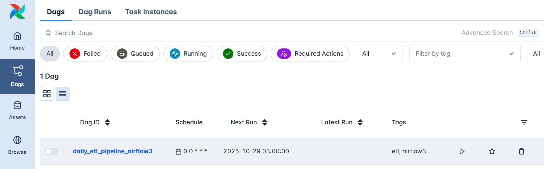
Click on it to open the DAG details, then trigger a manual run using the Play button.

The task currently running will turn blue, and once it completes successfully, it will turn green.

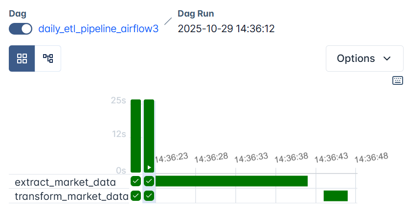
On the graph view, you will also see two tasks: extract_market_data and transform_market_data , connected in sequence showing success in each.

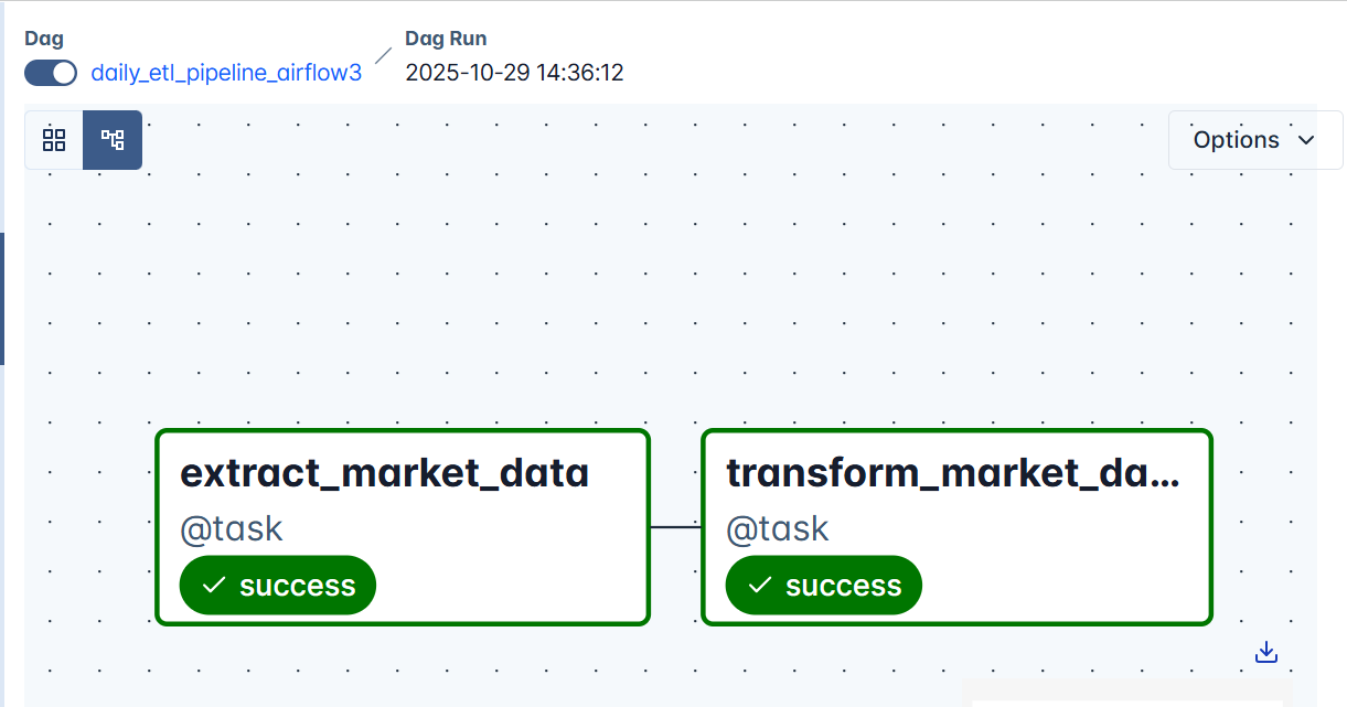
If a task encounters an issue, Airflow will automatically retry it up to three times (as defined in default_args). If it continues to fail after all retries, it will appear red, indicating that the task, and therefore the DAG run, has failed.

Inspecting Task Logs

Click on any task box (for example, transform_market_data), then click Task Instances.

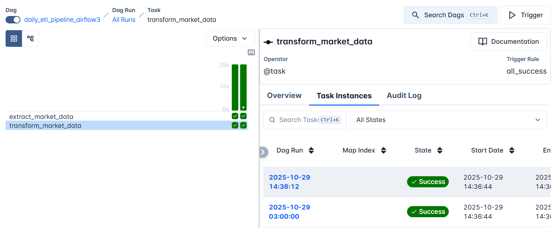
All DAG runs for the selected task will be listed here. Click on the latest run. This will open a detailed log of the task’s execution, an invaluable feature for debugging and understanding what’s happening under the hood.

In your log, you’ll see:

• The [EXTRACT] or [TRANSFORM] tags you printed in the code.

• Confirmation messages showing where your files were saved, e.g.:

  

  

These messages prove that your tasks executed correctly and help you trace your data through each stage of the pipeline.

Dynamic Task Mapping

As data engineers, we rarely process just one dataset; we usually work with many sources at once.

For example, instead of analyzing one market, you might process stock data from multiple exchanges or regions simultaneously.

In our current DAG, the extraction and transformation handle only a single dataset.

But what if we wanted to repeat that same process for several markets, say, us, europe, asia, and africa , all in parallel?

Writing a separate task for each region would make our DAG repetitive and hard to maintain.

That’s where Dynamic Task Mapping comes in.

It allows Airflow to create parallel tasks automatically at runtime based on input data such as lists, dictionaries, or query results.

Before editing the DAG, stop any running containers to ensure Airflow picks up your changes cleanly:

docker compose down -v

Now, extend your existing daily_etl_pipeline_airflow3 to handle multiple markets dynamically:

def daily_etl_pipeline():

    @task
    def extract_market_data(market: str):
        ...
    @task
    def transform_market_data(raw_file: str):
      ...

    # Define markets to process dynamically
    markets = ["us", "europe", "asia", "africa"]

    # Dynamically create parallel tasks
    raw_files = extract_market_data.expand(market=markets)
    transformed_files = transform_market_data.expand(raw_file=raw_files)

dag = daily_etl_pipeline()

By using .expand(), Airflow automatically generates multiple parallel task instances from a single function. You’ll notice the argument market passed into the extract_market_data() function. For that to work effectively, here’s the updated version of the extract_market_data() function:

@task
def extract_market_data(market: str):
        """Simulate extracting market data for a given region or market."""
        companies = ["Apple", "Amazon", "Google", "Microsoft", "Tesla", "Netflix"]
        records = []
        for company in companies:
            price = round(random.uniform(100, 1500), 2)
            change = round(random.uniform(-5, 5), 2)
            records.append({
                "timestamp": datetime.now().strftime("%Y-%m-%d %H:%M:%S"),
                "market": market,
                "company": company,
                "price_usd": price,
                "daily_change_percent": change,
            })

        df = pd.DataFrame(records)
        os.makedirs("/opt/airflow/tmp", exist_ok=True)
        raw_path = f"/opt/airflow/tmp/market_data_{market}.csv"
        df.to_csv(raw_path, index=False)
        print(f"[EXTRACT] Market data for {market} saved at {raw_path}")
        return raw_path

We also updated our transform_market_data() task to align with this dynamic setup:

@task
def transform_market_data(raw_file: str):
    """Clean and analyze each regional dataset."""
    df = pd.read_csv(raw_file)
    df["price_usd"] = pd.to_numeric(df["price_usd"], errors="coerce")
    df["daily_change_percent"] = pd.to_numeric(df["daily_change_percent"], errors="coerce")
    df_sorted = df.sort_values(by="daily_change_percent", ascending=False)

    top_gainers = df_sorted.head(3)
    top_losers = df_sorted.tail(3)

    transformed_path = raw_file.replace("market_data_", "transformed_")
    top_gainers.to_csv(transformed_path, index=False)
    print(f"[TRANSFORM] Transformed data saved at {transformed_path}")
    return transformed_path

Both extract_market_data() and transform_market_data() now work together dynamically:

• extract_market_data() generates a unique dataset per region (e.g., market_data_us.csv, market_data_europe.csv).
• transform_market_data() then processes each of those files individually and saves transformed versions (e.g., transformed_us.csv).

Generally:

• One extract task is created for each market (us, europe, asia, africa).
• Each extract’s output file becomes the input for its corresponding transform task.
• Airflow handles all the mapping logic automatically, no loops or manual duplication needed.

Let’s redeploy our containers by running docker compose up -d .

You’ll see this clearly in the Graph View, where the DAG fans out into several parallel branches, one per market.

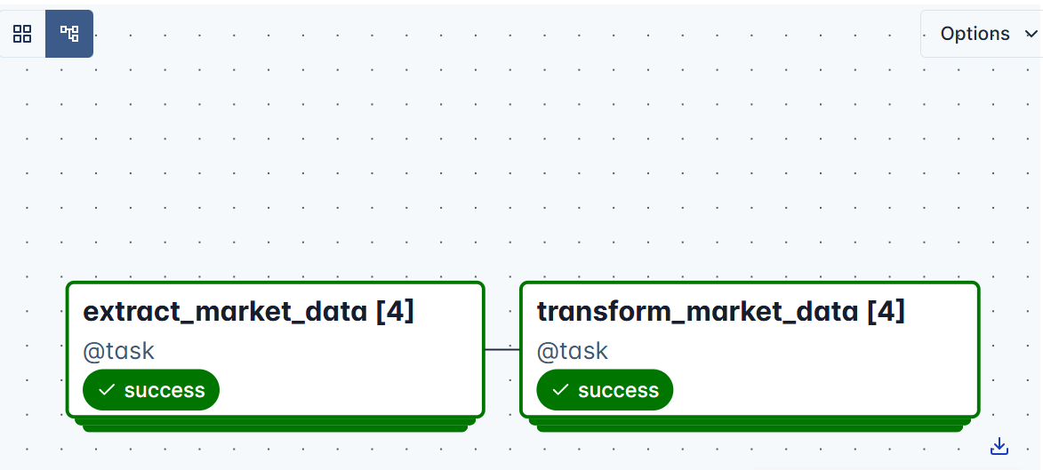
Each branch runs independently, and Airflow retries or logs failures per task as defined in default_args. You’ll notice that there are four task instances, which clearly correspond to the four market regions we processed.

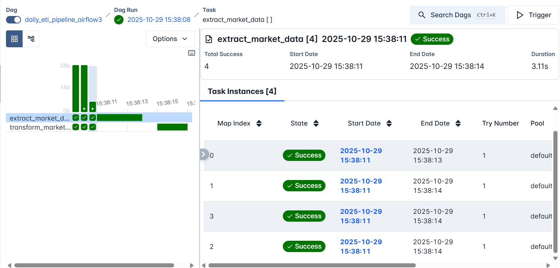
When you click any of the tasks, for example, extract_market_data , and open the logs, you’ll notice that the data for the corresponding market regions was extracted and saved independently.

Summary and What’s Next

We have built a complete foundation for working with Apache Airflow inside Docker. You learned how to deploy a fully functional Airflow environment using Docker Compose, understand its architecture, and configure it for clean, local development. We explored the Airflow Web UI, and used the TaskFlow API to create our first real workflow, a simple yet powerful ETL pipeline that extracts and transforms data automatically.

By extending it with Dynamic Task Mapping, we saw how Airflow can scale horizontally by processing multiple datasets in parallel, creating independent task instances for each region without duplicating code.

In Part Two, we’ll build on this foundation and introduce the Load phase of our ETL pipeline. You’ll connect Airflow to a local MySQL database, learn how to configure Connections through the Admin panel and environment variables. We’ll also integrate Git and Git Sync to automate DAG deployment and introduce CI/CD pipelines for version-controlled, collaborative Airflow workflows.

By the end of the next part, your environment will evolve from a development sandbox into a production-ready data orchestration system, capable of automating data ingestion, transformation, and loading with full observability, reliability, and continuous integration support.