Beginner Machine Learning Tutorial: Data Explorations and Prediction with Pandas, Scikit-learn, and Matplotlib
The Data Set
Before we dive into machine learning, we're going to explore a dataset, and figure out what might be interesting to predict. The dataset is from BoardGameGeek, and contains data on 80000 board games. Here's a single boardgame on the site. This information was kindly scraped into csv format by Sean Beck, and can be downloaded here. The dataset contains several data points about each board game. Here's a list of the interesting ones:
-
name-- name of the board game. -
playingtime-- the playing time (given by the manufacturer). -
minplaytime-- the minimum playing time (given by the manufacturer). -
maxplaytime-- the maximum playing time (given by the manufacturer). -
minage-- the minimum recommended age to play. -
users_rated-- the number of users who rated the game. -
average_rating-- the average rating given to the game by users. (0-10) -
total_weights-- Number of weights given by users.Weightis a subjective measure that is made up by BoardGameGeek. It's how "deep" or involved a game is. Here's a full explanation. -
average_weight-- the average of all the subjective weights (0-5).
Learn Python Programming: Introduction to Pandas
The first step in our exploration is to read in the data and print some quick summary statistics. In order to do this, we'll us the Pandas library. Pandas provides data structures and data analysis tools that make manipulating data in Python much quicker and more effective. The most common data structure is called a dataframe. A dataframe is an extension of a matrix, so we'll talk about what a matrix is before coming back to dataframes. Our data file looks like this (we removed some columns to make it easier to look at):
id,type,name,yearpublished,minplayers,maxplayers,playingtime
12333,boardgame,Twilight Struggle,2005,2,2,180
120677,boardgame,Terra Mystica,2012,2,5,150
This is in a format called csv, or comma-separated values, which you can read more about here. Each row of the data is a different board game, and different data points about each board game are separated by commas within the row. The first row is the header row, and describes what each data point is. The entire set of one data point, going down, is a column. We can easily conceptualize a csv file as a matrix:
_   1       2           3                   4
1   id      type        name                yearpublished
2   12333   boardgame   Twilight Struggle   2005
3   120677  boardgame   Terra Mystica       2012
We removed some of the columns here for display purposes, but you can still get a sense of how the data looks visually. A matrix is a two-dimensional data structure, with rows and columns. We can access elements in a matrix by position. The first row starts with id, the second row starts with 12333, and the third row starts with 120677. The first column is id, the second is type, and so on. Matrices in Python can be used via the NumPy library. A matrix has some downsides, though. You can't easily access columns and rows by name, and each column has to have the same datatype. This means that we can't effectively store our board game data in a matrix -- the name column contains strings, and the yearpublished column contains integers, which means that we can't store them both in the same matrix. A dataframe, on the other hand, can have different datatypes in each column. It has has a lot of built-in niceties for analyzing data as well, such as looking up columns by name. Pandas gives us access to these features, and generally makes working with data much simpler.
Reading in Our Data
We'll now read in our data from a csv file into a Pandas dataframe, using the read_csv method.
# Import the pandas library.
import pandas
# Read in the data.
games = pandas.read_csv("board_games.csv")
# Print the names of the columns in games.
print(games.columns)
Index(['id', 'type', 'name', 'yearpublished', 'minplayers', 'maxplayers','playingtime', 'minplaytime', 'maxplaytime', 'minage', 'users_rated', 'average_rating', 'bayes_average_rating', 'total_owners', 'total_traders', 'total_wanters', 'total_wishers', 'total_comments', 'total_weights', 'average_weight'],
dtype='object')The code above read the data in, and shows us all of the column names. The columns that are in the data but aren't listed above should be fairly self-explanatory.
print(games.shape)(81312, 20) We can also see the shape of the data, which shows that it has 81312 rows, or games, and 20 columns, or data points describing each game.
Plotting Our Target Variables
It could be interesting to predict the average score that a human would give to a new, unreleased, board game. This is stored in the average_rating column, which is the average of all the user ratings for a board game. Predicting this column could be useful to board game manufacturers who are thinking of what kind of game to make next, for instance. We can access a column is a dataframe with Pandas using games["average_rating"]. This will extract a single column from the dataframe. Let's plot a histogram of this column so we can visualize the distribution of ratings. We'll use Matplotlib to generate the visualization. Matplotlib is the main plotting infrastructure you'll discover as you learn Python programming, and most other plotting libraries, like seaborn and ggplot2 are built on top of Matplotlib. We import Matplotlib's plotting functions with import matplotlib.pyplot as plt. We can then draw and show plots.
# Import matplotlib
import matplotlib.pyplot as plt

# Make a histogram of all the ratings in the average_rating column.
plt.hist(games["average_rating"])

# Show the plot.plt.show() 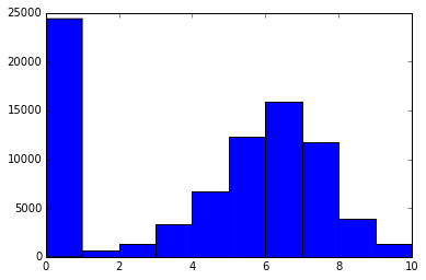
What we see here is that there are quite a few games with a 0 rating. There's a fairly normal distribution of ratings, with some right skew, and a mean rating around 6 (if you remove the zeros).
Exploring the 0 Ratings
Are there truly so many terrible games that were given a 0 rating? Or is something else happening? We'll need to dive into the data bit more to check on this. With Pandas, we can select subsets of data using Boolean series (vectors, or one column/row of data, are known as series in Pandas). Here's an example:
games[games["average_rating"] == 0] The code above will create a new dataframe, with only the rows in games where the value of the average_rating column equals 0. We can then index the resulting dataframe to get the values we want. There are two ways to index in Pandas — we can index by the name of the row or column, or we can index by position. Indexing by names looks like games["average_rating"] — this will return the whole average_rating column of games. Indexing by position looks like games.iloc[0] — this will return the whole first row of the dataframe. We can also pass in multiple index values at once — games.iloc[0,0] will return the first column in the first row of games. Read more about Pandas indexing here.
# Print the first row of all the games with zero scores.
# The .iloc method on dataframes allows us to index by position.
print(games[games["average_rating"] == 0].iloc[0])
# Print the first row of all the games with scores greater than 0.
print(games[games["average_rating"] > 0].iloc[0])
id 318
type boardgame
name Looney Leo
users_rated 0
average_rating 0
bayes_average_rating 0
Name: 13048, dtype: object
id 12333
type boardgame
name Twilight Struggle
users_rated 20113
average_rating 8.33774
bayes_average_rating 8.22186
Name: 0, dtype: object
This shows us that the main difference between a game with a 0 rating and a game with a rating above 0 is that the 0 rated game has no reviews. The users_rated column is 0. By filtering out any board games with 0 reviews, we can remove much of the noise.
Removing Games Without Reviews
# Remove any rows without user reviews.
games = games[games["users_rated"] > 0]
# Remove any rows with missing values.
games = games.dropna(axis=0)
We just filtered out all of the rows without user reviews. While we were at it, we also took out any rows with missing values. Many machine learning algorithms can't work with missing values, so we need some way to deal with them. Filtering them out is one common technique, but it means that we may potentially lose valuable data. Other techniques for dealing with missing data are listed here.
Clustering Games
We've seen that there may be distinct sets of games. One set (which we just removed) was the set of games without reviews. Another set could be a set of highly rated games. One way to figure out more about these sets of games is a technique called clustering. Clustering enables you to find patterns within your data easily by grouping similar rows (in this case, games), together. We'll use a particular type of clustering called k-means clustering. Scikit-learn has an excellent implementation of k-means clustering that we can use. Scikit-learn is the primary machine learning library in Python, and contains implementations of most common algorithms, including random forests, support vector machines, and logistic regression. Scikit-learn has a consistent API for accessing these algorithms.
# Import the kmeans clustering model.
from sklearn.cluster import KMeans

# Initialize the model with 2 parameters -- number of clusters and random state.
kmeans_model = KMeans(n_clusters=5, random_state=1)
# Get only the numeric columns from games.
good_columns = games._get_numeric_data()
# Fit the model using the good columns.
kmeans_model.fit(good_columns)
# Get the cluster assignments.
labels = kmeans_model.labels_
In order to use the clustering algorithm in Scikit-learn, we'll first intialize it using two parameters -- n_clusters defines how many clusters of games that we want, and random_state is a random seed we set in order to reproduce our results later. Here's more information on the implementation. We then only get the numeric columns from our dataframe. Most machine learning algorithms can't directly operate on text data, and can only take numbers as input. Getting only the numeric columns removes type and name, which aren't usable by the clustering algorithm. Finally, we fit our kmeans model to our data, and get the cluster assignment labels for each row.
Plotting Clusters
Now that we have cluster labels, let's plot the clusters. One sticking point is that our data has many columns -- it's outside of the realm of human understanding and physics to be able to visualize things in more than 3 dimensions. So we'll have to reduce the dimensionality of our data, without losing too much information. One way to do this is a technique called principal component analysis, or PCA. PCA takes multiple columns, and turns them into fewer columns while trying to preserve the unique information in each column. To simplify, say we have two columns, total_owners, and total_traders. There is some correlation between these two columns, and some overlapping information. PCA will compress this information into one column with new numbers while trying not to lose any information. We'll try to turn our board game data into two dimensions, or columns, so we can easily plot it out.
# Import the PCA model.
from sklearn.decomposition import PCA

# Create a PCA model.
pca_2 = PCA(2)
# Fit the PCA model on the numeric columns from earlier.
plot_columns = pca_2.fit_transform(good_columns)
# Make a scatter plot of each game, shaded according to cluster assignment.
plt.scatter(x=plot_columns[:,0], y=plot_columns[:,1], c=labels)
# Show the plot.
plt.show()
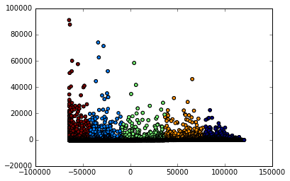
We first initialize a PCA model from Scikit-learn. PCA isn't a machine learning technique, but Scikit-learn also contains other models that are useful for performing machine learning. Dimensionality reduction techniques like PCA are widely used when preprocessing data for machine learning algorithms. We then turn our data into 2 columns, and plot the columns. When we plot the columns, we shade them according to their cluster assignment. The plot shows us that there are 5 distinct clusters. We could dive more into which games are in each cluster to learn more about what factors cause games to be clustered.
Figuring Out What to Predict
There are two things we need to determine before we jump into machine learning -- how we're going to measure error, and what we're going to predict. We thought earlier that average_rating might be good to predict on, and our exploration reinforces this notion. There are a variety of ways to measure error (many are listed here). Generally, when we're doing regression, and predicting continuous variables, we'll need a different error metric than when we're performing classification, and predicting discrete values. For this, we'll use mean squared error -- it's easy to calculate, and simple to understand. It shows us how far, on average, our predictions are from the actual values.
Finding Correlations
Now that we want to predict average_rating, let's see what columns might be interesting for our prediction. One way is to find the correlation between average_rating and each of the other columns. This will show us which other columns might predict average_rating the best. We can use the corr method on Pandas dataframes to easily find correlations. This will give us the correlation between each column and each other column. Since the result of this is a dataframe, we can index it and only get the correlations for the average_rating column.
games.corr()["average_rating"]
id                      0.304201
yearpublished           0.108461
minplayers             -0.032701
maxplayers             -0.008335
playingtime             0.048994
minplaytime             0.043985
maxplaytime             0.048994
minage                  0.210049
users_rated             0.112564
average_rating          1.000000
bayes_average_rating    0.231563
total_owners            0.137478
total_traders           0.119452
total_wanters           0.196566
total_wishers           0.171375
total_comments          0.123714
total_weights           0.109691
average_weight          0.351081
Name: average_rating, dtype: float64
We see that the average_weight and id columns correlate best to rating. ids are presumably assigned when the game is added to the database, so this likely indicates that games created later score higher in the ratings. Maybe reviewers were not as nice in the early days of BoardGameGeek, or older games were of lower quality. average_weight indicates the "depth" or complexity of a game, so it may be that more complex games are reviewed better.
Picking Predictor Columns
Before we get started predicting as we learn Python programming, let's only select the columns that are relevant when training our algorithm. We'll want to remove certain columns that aren't numeric. We'll also want to remove columns that can only be computed if you already know the average rating. Including these columns will destroy the purpose of the classifier, which is to predict the rating without any previous knowledge. Using columns that can only be computed with knowledge of the target can lead to overfitting, where your model is good in a training set, but doesn't generalize well to future data. The bayes_average_rating column appears to be derived from average_rating in some way, so let's remove it.
# Get all the columns from the dataframe.
columns = games.columns.tolist()
# Filter the columns to remove ones we don't want.
columns = [c for c in columns if c not in ["bayes_average_rating", "average_rating", "type", "name"]]

# Store the variable we'll be predicting on.
target = "average_rating"
Splitting Into Train and Test Sets
We want to be able to figure out how accurate an algorithm is using our error metrics. However, evaluating the algorithm on the same data it has been trained on will lead to overfitting. We want the algorithm to learn generalized rules to make predictions, not memorize how to make specific predictions. An example is learning math. If you memorize that 1+1=2, and 2+2=4, you'll be able to perfectly answer any questions about 1+1 and 2+2. You'll have 0 error. However, the second anyone asks you something outside of your training set where you know the answer, like 3+3, you won't be able to solve it. On the other hand, if you're able to generalize and learn addition, you'll make occasional mistakes because you haven't memorized the solutions -- maybe you'll get 3453 + 353535 off by one, but you'll be able to solve any addition problem thrown at you. If your error looks surprisingly low when you're training a machine learning algorithm, you should always check to see if you're overfitting. In order to prevent overfitting, we'll train our algorithm on a set consisting of 80% of the data, and test it on another set consisting of 20% of the data. To do this, we first randomly samply 80% of the rows to be in the training set, then put everything else in the testing set.
# Import a convenience function to split the sets.
from sklearn.cross_validation import train_test_split

# Generate the training set.  Set random_state to be able to replicate results.
train = games.sample(frac=0.8, random_state=1)
# Select anything not in the training set and put it in the testing set.
test = games.loc[~games.index.isin(train.index)]
# Print the shapes of both sets.
print(train.shape)
print(test.shape)
(45515, 20)
(11379, 20)
Above, we exploit the fact that every Pandas row has a unique index to select any row not in the training set to be in the testing set.
Fitting a Linear Regression
Linear regression is a powerful and commonly used machine learning algorithm. It predicts the target variable using linear combinations of the predictor variables. Let's say we have a 2 values, 3, and 4. A linear combination would be 3 * .5 + 4 * .5. A linear combination involves multiplying each number by a constant, and adding the results. You can read more here. Linear regression only works well when the predictor variables and the target variable are linearly correlated. As we saw earlier, a few of the predictors are correlated with the target, so linear regression should work well for us. We can use the linear regression implementation in Scikit-learn, just as we used the k-means implementation earlier.
# Import the linearregression model.
from sklearn.linear_model import LinearRegression

# Initialize the model class.
model = LinearRegression()
# Fit the model to the training data.
model.fit(train[columns], train[target])
When we fit the model, we pass in the predictor matrix, which consists of all the columns from the dataframe that we picked earlier. If you pass a list to a Pandas dataframe when you index it, it will generate a new dataframe with all of the columns in the list. We also pass in the target variable, which we want to make predictions for. The model learns the equation that maps the predictors to the target with minimal error.
Predicting Error
After we train the model, we can make predictions on new data with it. This new data has to be in the exact same format as the training data, or the model won't make accurate predictions. Our testing set is identical to the training set (except the rows contain different board games). We select the same subset of columns from the test set, and then make predictions on it.
# Import the scikit-learn function to compute error.
from sklearn.metrics import mean_squared_error
# Generate our predictions for the test set.
predictions = model.predict(test[columns])
# Compute error between our test predictions and the actual values.
mean_squared_error(predictions, test[target])
1.8239281903519875Once we have the predictions, we're able to compute error between the test set predictions and the actual values. Mean squared error has the formula \(\frac{1}{n}\sum_{i=1}^{n}(y_i - \hat{y}_i)^{2}\) . Basically, we subtract each predicted value from the actual value, square the differences, and add them together. Then we divide the result by the total number of predicted values. This will give us the average error for each prediction.
Trying a Different Model
One of the nice things about Scikit-learn is that it enables us to try more powerful algorithms very easily. One such algorithm is called random forest. The random forest algorithm can find nonlinearities in data that a linear regression wouldn't be able to pick up on. Say, for example, that if the minage of a game, is less than 5, the rating is low, if it's 5-10, it's high, and if it is between 10-15, it is low. A linear regression algorithm wouldn't be able to pick up on this because there isn't a linear relationship between the predictor and the target. Predictions made with a random forest usually have less error than predictions made by linear regression.
# Import the random forest model.
from sklearn.ensemble import RandomForestRegressor

# Initialize the model with some parameters.
model = RandomForestRegressor(n_estimators=100, min_samples_leaf=10, random_state=1)
# Fit the model to the data.
model.fit(train[columns], train[target])
# Make predictions.
predictions = model.predict(test[columns])
# Compute the error.
mean_squared_error(predictions, test[target])
1.4144905030983794Further Exploration
We've managed to go from data in csv format to making predictions. Here are some ideas for further exploration:
- Try a support vector machine.
- Try ensembling multiple models to create better predictions.
-
Try predicting a different column, such as
average_weight. - Generate features from the text, such as length of the name of the game, number of words, etc.
Learn data skills 10x faster
Join 1M+ learners
Enroll for free