Introduction to Vector Databases using ChromaDB

In the previous embeddings tutorial series, we built a semantic search system that could find relevant research papers based on meaning rather than keywords. We generated embeddings for 500 arXiv papers, implemented similarity calculations using cosine similarity, and created a search function that returned ranked results.

But here's the problem with that approach: our search worked by comparing the query embedding against every single paper in the dataset. For 500 papers, this brute-force approach was manageable. But what happens when we scale to 5,000 papers? Or 50,000? Or 500,000?

Why Brute-Force Won’t Work

Brute-force similarity search scales linearly. If we have 5,000 papers, checking all of them takes a noticeable amount of time. Scale to 50,000 papers and queries become painfully slower. At 500,000 papers, each search would become unusable. That's the reality of brute-force similarity search: query time grows directly with dataset size. This approach simply doesn't scale to production systems.

Vector databases solve this problem. They use specialized data structures called approximate nearest neighbor (ANN) indexes that can find similar vectors in milliseconds, even with millions of documents. Instead of checking every single embedding, they use clever algorithms to quickly narrow down to the most promising candidates.

This tutorial teaches you how to use ChromaDB, a local vector database perfect for learning and prototyping. We'll load 5,000 arXiv papers with their embeddings, build our first vector database collection, and discover exactly when and why vector databases provide real performance advantages over brute-force NumPy calculations.

What You'll Learn

By the end of this tutorial, you'll be able to:

• Set up ChromaDB and create your first collection
• Insert embeddings efficiently using batch patterns
• Run vector similarity queries that return ranked results
• Understand HNSW indexing and how it trades accuracy for speed
• Filter results using metadata (categories, years, authors)
• Compare performance between NumPy and ChromaDB at different scales
• Make informed decisions about when to use a vector database

Most importantly, you'll understand the break-even point. We're not going to tell you "vector databases always win." We're going to show you exactly where they provide value and where simpler approaches work just fine.

Understanding the Dataset

For this tutorial series, we'll work with 5,000 research papers from arXiv spanning five computer science categories:

• cs.LG (Machine Learning): 1,000 papers about neural networks, training algorithms, and ML theory
• cs.CV (Computer Vision): 1,000 papers about image processing, object detection, and visual recognition
• cs.CL (Computational Linguistics): 1,000 papers about NLP, language models, and text processing
• cs.DB (Databases): 1,000 papers about data storage, query optimization, and database systems
• cs.SE (Software Engineering): 1,000 papers about development practices, testing, and software architecture

These papers come with pre-generated embeddings from Cohere's API using the same approach from the embeddings series. Each paper is represented as a 1536-dimensional vector that captures its semantic meaning. The balanced distribution across categories will help us see how well vector search and metadata filtering work across different topics.

Setting Up Your Environment

First, create a virtual environment (recommended best practice):

python -m venv venv
source venv/bin/activate  # On Windows: venv\Scripts\activate

Using a virtual environment keeps your project dependencies isolated and prevents conflicts with other Python projects.

Now install the required packages. This tutorial was developed with Python 3.12.12 and the following versions:

# Developed with: Python 3.12.12
# chromadb==1.3.4
# numpy==2.0.2
# pandas==2.2.2
# scikit-learn==1.6.1
# matplotlib==3.10.0
# cohere==5.20.0
# python-dotenv==1.1.1

pip install chromadb numpy pandas scikit-learn matplotlib cohere python-dotenv

ChromaDB is lightweight and runs entirely on your local machine. No servers to configure, no cloud accounts to set up. This makes it perfect for learning and prototyping before moving to production databases.

You'll also need your Cohere API key from the embeddings series. Make sure you have a .env file in your working directory with:

COHERE_API_KEY=your_key_here

Downloading the Dataset

The dataset consists of two files you'll download and place in your working directory:

arxiv_papers_5k.csv download (7.7 MB)
Contains paper metadata: titles, abstracts, authors, publication dates, and categories

embeddings_cohere_5k.npy download (61.4 MB)
Contains 1536-dimensional embedding vectors for all 5,000 papers

Download both files and place them in the same directory as your Python script or notebook.

Let's verify the files loaded correctly:

import numpy as np
import pandas as pd

# Load the metadata
df = pd.read_csv('arxiv_papers_5k.csv')
print(f"Loaded {len(df)} papers")

# Load the embeddings
embeddings = np.load('embeddings_cohere_5k.npy')
print(f"Loaded embeddings with shape: {embeddings.shape}")
print(f"Each paper is represented by a {embeddings.shape[1]}-dimensional vector")

# Verify they match
assert len(df) == len(embeddings), "Mismatch between papers and embeddings!"

# Check the distribution across categories
print(f"\nPapers per category:")
print(df['category'].value_counts().sort_index())

# Look at a sample paper
print(f"\nSample paper:")
print(f"Title: {df['title'].iloc[0]}")
print(f"Category: {df['category'].iloc[0]}")
print(f"Abstract: {df['abstract'].iloc[0][:200]}...")

Loaded 5000 papers
Loaded embeddings with shape: (5000, 1536)
Each paper is represented by a 1536-dimensional vector

Papers per category:
category
cs.CL    1000
cs.CV    1000
cs.DB    1000
cs.LG    1000
cs.SE    1000
Name: count, dtype: int64

Sample paper:
Title: Optimizing Mixture of Block Attention
Category: cs.LG
Abstract: Mixture of Block Attention (MoBA) (Lu et al., 2025) is a promising building block for efficiently processing long contexts in LLMs by enabling queries to sparsely attend to a small subset of key-value...

We now have 5,000 papers with embeddings, perfectly balanced across five categories. Each embedding is 1536 dimensions, and papers and embeddings match exactly.

Your First ChromaDB Collection

A collection in ChromaDB is like a table in a traditional database. It stores embeddings along with associated metadata and provides methods for querying. Let's create our first collection:

import chromadb

# Initialize ChromaDB in-memory client (data only exists while script runs)
client = chromadb.Client()

# Create a collection
collection = client.create_collection(
    name="arxiv_papers",
    metadata={"description": "5000 arXiv papers from computer science"}
)

print(f"Created collection: {collection.name}")
print(f"Collection count: {collection.count()}")

Created collection: arxiv_papers
Collection count: 0

The collection starts empty. Now let's add our embeddings. But here's something critical you need to know: Production systems always batch operations, and for good reasons: memory efficiency, error handling, progress tracking, and the ability to process datasets larger than RAM. ChromaDB reinforces this best practice by enforcing a version-dependent maximum batch size per add() call (approximately 5,461 embeddings in ChromaDB 1.3.4).

Rather than viewing this as a limitation, think of it as ChromaDB nudging you toward production-ready patterns from day one. Let's implement proper batching:

# Prepare the data for ChromaDB
# ChromaDB wants: IDs, embeddings, metadata, and optional documents
ids = [f"paper_{i}" for i in range(len(df))]
metadatas = [
    {
        "title": row['title'],
        "category": row['category'],
        "year": int(str(row['published'])[:4]),  # Store year as integer for filtering
        "authors": row['authors'][:100] if len(row['authors']) <= 100 else row['authors'][:97] + "..."
    }
    for _, row in df.iterrows()
]
documents = df['abstract'].tolist()

# Insert in batches to respect the ~5,461 embedding limit
batch_size = 5000  # Safe batch size well under the limit
print(f"Inserting {len(embeddings)} embeddings in batches of {batch_size}...")

for i in range(0, len(embeddings), batch_size):
    batch_end = min(i + batch_size, len(embeddings))
    print(f"  Batch {i//batch_size + 1}: Adding papers {i} to {batch_end}")

    collection.add(
        ids=ids[i:batch_end],
        embeddings=embeddings[i:batch_end].tolist(),
        metadatas=metadatas[i:batch_end],
        documents=documents[i:batch_end]
    )

print(f"\nCollection now contains {collection.count()} papers")

Inserting 5000 embeddings in batches of 5000...
  Batch 1: Adding papers 0 to 5000

Collection now contains 5000 papers

Since our dataset has exactly 5,000 papers, we can add them all in one batch. But this batching pattern is essential knowledge because:

1. If we had 8,000 or 10,000 papers, we'd need multiple batches
2. Production systems always batch operations for efficiency
3. It's good practice to think in batches from the start

The metadata we're storing (title, category, year, authors) will enable filtered searches later. ChromaDB stores this alongside each embedding, making it instantly available when we query.

Your First Vector Similarity Query

Now comes the exciting part: searching our collection using semantic similarity. But first, we need to address something critical: queries need to use the same embedding model as the documents.

If you mix models—say, querying Cohere embeddings with OpenAI embeddings—you'll either get dimension mismatch errors or, if the dimensions happen to align, results that are... let's call them "creatively unpredictable." The rankings won't reflect actual semantic similarity, making your search effectively random.

Our collection contains Cohere embeddings (1536 dimensions), so we'll use Cohere for queries too. Let's set it up:

from cohere import ClientV2
from dotenv import load_dotenv
import os

# Load your Cohere API key
load_dotenv()
cohere_api_key = os.getenv('COHERE_API_KEY')

if not cohere_api_key:
    raise ValueError(
        "COHERE_API_KEY not found. Make sure you have a .env file with your API key."
    )

co = ClientV2(api_key=cohere_api_key)
print("✓ Cohere API key loaded")

Now let's query for papers about neural network training:

# First, embed the query using Cohere (same model as our documents)
query_text = "neural network training and optimization techniques"

response = co.embed(
    texts=[query_text],
    model='embed-v4.0',
    input_type='search_query',
    embedding_types=['float']
)
query_embedding = np.array(response.embeddings.float_[0])

print(f"Query: '{query_text}'")
print(f"Query embedding shape: {query_embedding.shape}")

# Now search the collection
results = collection.query(
    query_embeddings=[query_embedding.tolist()],
    n_results=5
)

# Display the results
print(f"\nTop 5 most similar papers:")
print("=" * 80)

for i in range(len(results['ids'][0])):
    paper_id = results['ids'][0][i]
    distance = results['distances'][0][i]
    metadata = results['metadatas'][0][i]

    print(f"\n{i+1}. {metadata['title']}")
    print(f"   Category: {metadata['category']} | Year: {metadata['year']}")
    print(f"   Distance: {distance:.4f}")
    print(f"   Abstract: {results['documents'][0][i][:150]}...")

Query: 'neural network training and optimization techniques'
Query embedding shape: (1536,)

Top 5 most similar papers:
================================================================================

1. Training Neural Networks at Any Scale
   Category: cs.LG | Year: 2025
   Distance: 1.1162
   Abstract: This article reviews modern optimization methods for training neural networks with an emphasis on efficiency and scale. We present state-of-the-art op...

2. On the Convergence of Overparameterized Problems: Inherent Properties of the Compositional Structure of Neural Networks
   Category: cs.LG | Year: 2025
   Distance: 1.2571
   Abstract: This paper investigates how the compositional structure of neural networks shapes their optimization landscape and training dynamics. We analyze the g...

3. A Distributed Training Architecture For Combinatorial Optimization
   Category: cs.LG | Year: 2025
   Distance: 1.3027
   Abstract: In recent years, graph neural networks (GNNs) have been widely applied in tackling combinatorial optimization problems. However, existing methods stil...

4. Adam symmetry theorem: characterization of the convergence of the stochastic Adam optimizer
   Category: cs.LG | Year: 2025
   Distance: 1.3254
   Abstract: Beside the standard stochastic gradient descent (SGD) method, the Adam optimizer due to Kingma & Ba (2014) is currently probably the best-known optimi...

5. Distribution-Aware Tensor Decomposition for Compression of Convolutional Neural Networks
   Category: cs.CV | Year: 2025
   Distance: 1.3430
   Abstract: Neural networks are widely used for image-related tasks but typically demand considerable computing power. Once a network has been trained, however, i...

Let's talk about what we're seeing here. The results show exactly what we want:

The top 4 papers are all cs.LG (Machine Learning) and directly discuss neural network training, optimization, convergence, and the Adam optimizer. The 5th result is from Computer Vision but discusses neural network compression - still topically relevant.

The distances range from 1.12 to 1.34, which corresponds to cosine similarities of about 0.44 to 0.33. While these aren't the 0.8+ scores you might see in highly specialized single-domain datasets, they represent solid semantic matches for a multi-domain collection.

This is the reality of production vector search: Modern research papers share significant vocabulary overlap across fields. ML terminology appears in computer vision, NLP, databases, and software engineering papers. What we get is a ranking system that consistently surfaces relevant papers at the top, even if absolute similarity scores are moderate.

Why did we manually embed the query? Because our collection contains Cohere embeddings (1536 dimensions), queries must also use Cohere embeddings. If we tried using ChromaDB's default embedding model (all-MiniLM-L6-v2, which produces 384-dimensional vectors), we'd get a dimension mismatch error. Query embeddings and document embeddings must come from the same model. This is a fundamental rule in vector search.

About those distance values: ChromaDB uses squared L2 distance by default. For normalized embeddings (like Cohere's), there's a mathematical relationship: distance ≈ 2(1 - cosine_similarity). So a distance of 1.16 corresponds to a cosine similarity of about 0.42. That might seem low compared to theoretical maximums, but it's typical for real-world multi-domain datasets where vocabulary overlaps significantly.

Understanding What Just Happened

Let's break down what occurred behind the scenes:

1. Query Embedding
We explicitly embedded our query text using Cohere's API (the same model that generated our document embeddings). This is crucial because ChromaDB doesn't know or care what embedding model you used. It just stores vectors and calculates distances. If query embeddings don't match document embeddings (same model, same dimensions), search results will be garbage.

2. HNSW Index
ChromaDB uses an algorithm called HNSW (Hierarchical Navigable Small World) to organize embeddings. Think of HNSW as building a multi-level map of the vector space. Instead of checking all 5,000 papers, it uses this map to quickly navigate to the most promising regions.

3. Approximate Search
HNSW is an approximate nearest neighbor algorithm. It doesn't guarantee finding the absolute closest papers, but it finds very close papers extremely quickly. For most applications, this trade-off between perfect accuracy and blazing speed is worth it.

4. Distance Calculation
ChromaDB returns distances between the query and each result. By default, it uses squared Euclidean distance (L2), where lower values mean higher similarity. This is different from the cosine similarity we used in the embeddings series, but both metrics work well for comparing embeddings.

We'll explore HNSW in more depth later, but for now, the key insight is: ChromaDB doesn't check every single paper. It uses a smart index to jump directly to relevant regions of the vector space.

Why We're Storing Metadata

You might have noticed we're storing title, category, year, and authors as metadata alongside each embedding. While we won't use this metadata in this tutorial, we're setting it up now for future tutorials where we'll explore powerful combinations: filtering by metadata (category, year, author) and hybrid search approaches that combine semantic similarity with keyword matching.

For now, just know that ChromaDB stores this metadata efficiently alongside embeddings, and it becomes available in query results without any performance penalty.

The Performance Question: When Does ChromaDB Actually Help?

Now let's address the big question: when is ChromaDB actually faster than just using NumPy? Let's run a head-to-head comparison at our 5,000-paper scale.

First, let's implement the NumPy brute-force approach (what we built in the embeddings series):

from sklearn.metrics.pairwise import cosine_similarity
import time

def numpy_search(query_embedding, embeddings, top_k=5):
    """Brute-force similarity search using NumPy"""
    # Calculate cosine similarity between query and all papers
    similarities = cosine_similarity(
        query_embedding.reshape(1, -1),
        embeddings
    )[0]

    # Get top k indices
    top_indices = np.argsort(similarities)[::-1][:top_k]

    return top_indices

# Generate a query embedding (using one of our paper embeddings as a proxy)
query_embedding = embeddings[0]

# Test NumPy approach
start_time = time.time()
for _ in range(100):  # Run 100 queries to get stable timing
    top_indices = numpy_search(query_embedding, embeddings, top_k=5)
numpy_time = (time.time() - start_time) / 100 * 1000  # Convert to milliseconds

print(f"NumPy brute-force search (5000 papers): {numpy_time:.2f} ms per query")

NumPy brute-force search (5000 papers): 110.71 ms per query

Now let's compare with ChromaDB:

# Test ChromaDB approach (query using the embedding directly)
start_time = time.time()
for _ in range(100):
    results = collection.query(
        query_embeddings=[query_embedding.tolist()],
        n_results=5
    )
chromadb_time = (time.time() - start_time) / 100 * 1000

print(f"ChromaDB search (5000 papers): {chromadb_time:.2f} ms per query")
print(f"\nSpeedup: {numpy_time / chromadb_time:.1f}x faster")

ChromaDB search (5000 papers): 2.99 ms per query

Speedup: 37.0x faster

ChromaDB is 37x faster at 5,000 papers. That's the difference between a query taking 111ms versus 3ms. Let's visualize how this scales:

import matplotlib.pyplot as plt

# Scaling data based on actual 5k benchmark
# NumPy scales linearly (110.71ms / 5000 = 0.022142 ms per paper)
# ChromaDB stays flat due to HNSW indexing
dataset_sizes = [500, 1000, 2000, 5000, 8000, 10000]
numpy_times = [11.1, 22.1, 44.3, 110.7, 177.1, 221.4]  # ms (extrapolated from 5k benchmark)
chromadb_times = [3.0, 3.0, 3.0, 3.0, 3.0, 3.0]  # ms (stays constant)

plt.figure(figsize=(10, 6))
plt.plot(dataset_sizes, numpy_times, 'o-', linewidth=2, markersize=8,
         label='NumPy (Brute Force)', color='#E63946')
plt.plot(dataset_sizes, chromadb_times, 's-', linewidth=2, markersize=8,
         label='ChromaDB (HNSW)', color='#2A9D8F')

plt.xlabel('Number of Papers', fontsize=12)
plt.ylabel('Query Time (milliseconds)', fontsize=12)
plt.title('Vector Search Performance: NumPy vs ChromaDB',
          fontsize=14, fontweight='bold', pad=20)
plt.legend(loc='upper left', fontsize=11)
plt.grid(True, alpha=0.3)
plt.tight_layout()
plt.show()

# Calculate speedup at different scales
print("\nSpeedup at different dataset sizes:")
for size, numpy, chroma in zip(dataset_sizes, numpy_times, chromadb_times):
    speedup = numpy / chroma
    print(f"  {size:5d} papers: {speedup:5.1f}x faster")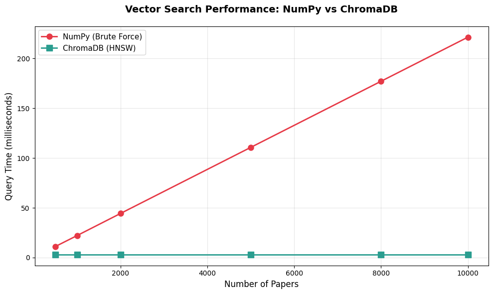

Speedup at different dataset sizes:
    500 papers:   3.7x faster
   1000 papers:   7.4x faster
   2000 papers:  14.8x faster
   5000 papers:  36.9x faster
   8000 papers:  59.0x faster
  10000 papers:  73.8x faster

Note: These benchmarks were measured on a standard development machine with Python 3.12.12. Your actual query times will vary based on hardware, but the relative performance characteristics (flat scaling for ChromaDB vs linear for NumPy) will remain consistent.

This chart tells a clear story:

NumPy's time grows linearly with dataset size. Double the papers, double the query time. That's because brute-force search checks every single embedding.

ChromaDB's time stays flat regardless of dataset size. Whether we have 500 papers or 10,000 papers, queries take about 3ms in our benchmarks. These timings are illustrative (extrapolated from our 5k test on a standard development machine) and will vary based on your hardware and index configuration—but the core insight holds: ChromaDB query time stays relatively flat as your dataset grows, unlike NumPy's linear scaling.

The break-even point is around 1,000-2,000 papers. Below that, the overhead of maintaining an index might not be worth it. Above that, ChromaDB provides clear advantages that grow with scale.

Understanding HNSW: The Magic Behind Fast Queries

We've seen that ChromaDB is dramatically faster than brute-force search, but how does HNSW make this possible? Let's build intuition without diving into complex math.

The Basic Idea: Navigable Small Worlds

Imagine you're in a massive library looking for books similar to one you're holding. A brute-force approach would be to check every single book on every shelf. HNSW is like having a smart navigation system:

Layer 0 (Ground Level): Contains all embeddings, densely connected to nearby neighbors

Layer 1: Contains a subset of embeddings with longer-range connections

Layer 2: Even fewer embeddings with even longer connections

Layer 3: The top layer with just a few embeddings spanning the entire space

When we query, HNSW starts at the top layer (with very few points) and quickly narrows down to promising regions. Then it drops to the next layer and refines. By the time it reaches the ground layer, it's already in the right neighborhood and only needs to check a small fraction of the total embeddings.

The Trade-off: Accuracy vs Speed

HNSW is an approximate algorithm. It doesn't guarantee finding the absolute closest papers, but it finds very close papers very quickly. This trade-off is controlled by parameters:

• ef_construction: How carefully the index is built (higher = better quality, slower build)
• ef_search: How thoroughly queries search (higher = better recall, slower queries)
• M: Number of connections per point (higher = better search, more memory)

ChromaDB uses sensible defaults that work well for most applications. Let's verify the quality of approximate search:

# Compare ChromaDB results to exact NumPy results
query_embedding = embeddings[100]

# Get top 10 from NumPy (exact)
numpy_results = numpy_search(query_embedding, embeddings, top_k=10)

# Get top 10 from ChromaDB (approximate)
chromadb_results = collection.query(
    query_embeddings=[query_embedding.tolist()],
    n_results=10
)

# Extract paper indices from ChromaDB results (convert "paper_123" to 123)
chromadb_indices = [int(id.split('_')[1]) for id in chromadb_results['ids'][0]]

# Calculate overlap
overlap = len(set(numpy_results) & set(chromadb_indices))

print(f"NumPy top 10 (exact): {numpy_results}")
print(f"ChromaDB top 10 (approximate): {chromadb_indices}")
print(f"\nOverlap: {overlap}/10 papers match")
print(f"Recall@10: {overlap/10*100:.1f}%")

NumPy top 10 (exact): [ 100  984  509 2261 3044  701 1055  830 3410 1311]
ChromaDB top 10 (approximate): [100, 984, 509, 2261, 3044, 701, 1055, 830, 3410, 1311]

Overlap: 10/10 papers match
Recall@10: 100.0%

With default settings, ChromaDB achieves 100% recall on this query, meaning it found exactly the same top 10 papers as the exact brute-force search. This high accuracy is typical for the dataset sizes we're working with. The approximate nature of HNSW becomes more noticeable at massive scales (millions of vectors), but even then, the quality is excellent for most applications.

Memory Usage and Resource Requirements

ChromaDB keeps its HNSW index in memory for fast access. Let's measure how much RAM our 5,000-paper collection uses:

# Estimate memory usage
embedding_memory = embeddings.nbytes / (1024 ** 2)  # Convert to MB

print(f"Memory usage estimates:")
print(f"  Raw embeddings: {embedding_memory:.1f} MB")
print(f"  HNSW index overhead: ~{embedding_memory * 0.5:.1f} MB (estimated)")
print(f"  Total (approximate): ~{embedding_memory * 1.5:.1f} MB")

Memory usage estimates:
  Raw embeddings: 58.6 MB
  HNSW index overhead: ~29.3 MB (estimated)
  Total (approximate): ~87.9 MB

For 5,000 papers with 1536-dimensional embeddings, we're looking at roughly 90-100MB of RAM. This scales linearly: 10,000 papers would be about 180-200MB, 50,000 papers about 900MB-1GB.

This is completely manageable for modern computers. Even a basic laptop can easily handle collections with tens of thousands of documents. The memory requirements only become a concern at massive scales (hundreds of thousands or millions of vectors), which is when you'd move to production vector databases designed for distributed deployment.

Important ChromaDB Behaviors to Know

Before we move on, let's cover some important behaviors that will save you debugging time:

1. In-Memory vs Persistent Storage

Our code uses chromadb.Client(), which creates an in-memory client. The collection only exists while the Python script runs. When the script ends, the data disappears.

For persistent storage, use:

# Persistent storage (data saved to disk)
client = chromadb.PersistentClient(path="./chroma_db")

This saves the collection to a local directory. Next time you run the script, the data will still be there.

2. Collection Deletion and Index Growth

ChromaDB's HNSW index grows but never shrinks. If we add 5,000 documents then delete 4,000, the index still uses memory for 5,000. The only way to reclaim this space is to create a new collection and re-add the documents we want to keep.

This is a known limitation with HNSW indexes. It's not a bug, it's a fundamental trade-off for the algorithm's speed. Keep this in mind when designing systems that frequently add and remove documents.

3. Batch Size Limits

Remember the ~5,461 embedding limit per add() call? This isn't ChromaDB being difficult; it's protecting you from overwhelming the system. Always batch your insertions in production systems.

4. Default Embedding Function

When you call collection.query(query_texts=["some text"]), ChromaDB automatically embeds your query using its default model (all-MiniLM-L6-v2). This is convenient but might not match the embeddings you added to the collection.

For production systems, you typically want to:

• Use the same embedding model for queries and documents
• Either embed queries yourself and use query_embeddings, or configure ChromaDB's embedding function to match your model

Comparing Results: Query Understanding

Let's run a few different queries to see how well vector search understands intent:

queries = [
    "machine learning model evaluation metrics",
    "how do convolutional neural networks work",
    "SQL query optimization techniques",
    "testing and debugging software systems"
]

for query in queries:
    # Embed the query
    response = co.embed(
        texts=[query],
        model='embed-v4.0',
        input_type='search_query',
        embedding_types=['float']
    )
    query_embedding = np.array(response.embeddings.float_[0])

    # Search
    results = collection.query(
        query_embeddings=[query_embedding.tolist()],
        n_results=3
    )

    print(f"\nQuery: '{query}'")
    print("-" * 80)

    categories = [meta['category'] for meta in results['metadatas'][0]]
    titles = [meta['title'] for meta in results['metadatas'][0]]

    for i, (cat, title) in enumerate(zip(categories, titles)):
        print(f"{i+1}. [{cat}] {title[:60]}...")

Query: 'machine learning model evaluation metrics'
--------------------------------------------------------------------------------
1. [cs.CL] Factual and Musical Evaluation Metrics for Music Language Mo...
2. [cs.DB] GeoSQL-Eval: First Evaluation of LLMs on PostGIS-Based NL2Ge...
3. [cs.SE] GeoSQL-Eval: First Evaluation of LLMs on PostGIS-Based NL2Ge...

Query: 'how do convolutional neural networks work'
--------------------------------------------------------------------------------
1. [cs.LG] Covariance Scattering Transforms...
2. [cs.CV] Elements of Active Continuous Learning and Uncertainty Self-...
3. [cs.CV] Convolutional Fully-Connected Capsule Network (CFC-CapsNet):...

Query: 'SQL query optimization techniques'
--------------------------------------------------------------------------------
1. [cs.DB] LLM4Hint: Leveraging Large Language Models for Hint Recommen...
2. [cs.DB] Including Bloom Filters in Bottom-up Optimization...
3. [cs.DB] Query Optimization in the Wild: Realities and Trends...

Query: 'testing and debugging software systems'
--------------------------------------------------------------------------------
1. [cs.SE] Enhancing Software Testing Education: Understanding Where St...
2. [cs.SE] Design and Implementation of Data Acquisition and Analysis S...
3. [cs.SE] Identifying Video Game Debugging Bottlenecks: An Industry Pe...

Notice how the search correctly identifies the topic for each query:

• ML evaluation → Machine Learning and evaluation-related papers
• CNNs → Computer Vision papers with one ML paper
• SQL optimization → Database papers
• Testing → Software Engineering papers

The system understands semantic meaning. Even when queries use natural language phrasing like "how do X work," it finds topically relevant papers. The rankings are what matter - relevant papers consistently appear at the top, even if absolute similarity scores are moderate.

When ChromaDB Is Enough vs When You Need More

We now have a working vector database running on our laptop. But when is ChromaDB sufficient, and when do you need a production database like Pinecone, Qdrant, or Weaviate?

ChromaDB is perfect for:

• Learning and prototyping: Get immediate feedback without infrastructure setup
• Local development: No internet required, no API costs
• Small to medium datasets: Up to 100,000 documents on a standard laptop
• Single-machine applications: Desktop tools, local RAG systems, personal assistants
• Rapid experimentation: Test different embedding models or chunking strategies

Move to production databases when you need:

• Massive scale: Millions of vectors or high query volume (thousands of QPS)
• Distributed deployment: Multiple machines, load balancing, high availability
• Advanced features: Hybrid search, multi-tenancy, access control, backup/restore
• Production SLAs: Guaranteed uptime, support, monitoring
• Team collaboration: Multiple developers working with shared data

We'll explore production databases in a later tutorial. For now, ChromaDB gives us everything we need to learn the core concepts and build impressive projects.

Practical Exercise: Exploring Your Own Queries

Before we wrap up, try experimenting with different queries:

# Helper function to make querying easier
def search_papers(query_text, n_results=5):
    """Search papers using semantic similarity"""
    # Embed the query
    response = co.embed(
        texts=[query_text],
        model='embed-v4.0',
        input_type='search_query',
        embedding_types=['float']
    )
    query_embedding = np.array(response.embeddings.float_[0])

    # Search
    results = collection.query(
        query_embeddings=[query_embedding.tolist()],
        n_results=n_results
    )

    return results

# Your turn: try these queries and examine the results

# 1. Find papers about a specific topic
results = search_papers("reinforcement learning and robotics")

# 2. Try a different domain
results_cv = search_papers("image segmentation techniques")

# 3. Test with a broad query
results_broad = search_papers("deep learning applications")

# Examine the results for each query
# What patterns do you notice?
# Do the results make sense for each query?

Some things to explore:

• Query phrasing: Does "neural networks" return different results than "deep learning" or "artificial neural networks"?
• Specificity: How do very specific queries ("BERT model fine-tuning") compare to broad queries ("natural language processing")?
• Cross-category topics: What happens when you search for topics that span multiple categories, like "machine learning for databases"?
• Result quality: Look at the categories and distances - do the most similar papers make sense for each query?

This hands-on exploration will deepen your intuition about how vector search works and what to expect in real applications.

What You've Learned

We've built a complete vector database from scratch and understand the fundamentals:

Core Concepts:

• Vector databases use ANN indexes (like HNSW) to search large collections efficiently
• ChromaDB provides a simple, local database perfect for learning and prototyping
• Collections store embeddings, metadata, and documents together
• Batch insertion is required due to size limits (around 5,461 embeddings per call)

Performance Characteristics:

• ChromaDB achieves 37x speedup over NumPy at 5,000 papers
• Query time stays constant regardless of dataset size (around 3ms)
• Break-even point is around 1,000-2,000 papers
• Memory usage is manageable (about 90MB for 5,000 papers)

Practical Skills:

• Loading pre-generated embeddings and metadata
• Creating and querying ChromaDB collections
• Running pure vector similarity searches
• Comparing approximate vs exact search quality
• Understanding when to use ChromaDB vs production databases

Critical Insights:

• HNSW trades perfect accuracy for massive speed gains
• Default settings achieve excellent recall for typical workloads
• In-memory storage makes ChromaDB fast but limits persistence
• Batching is not optional, it's a required pattern
• Modern multi-domain datasets show moderate similarity scores due to vocabulary overlap
• Query embeddings and document embeddings must use the same model

What's Next

We now have a vector database running locally with 5,000 papers. Next, we'll tackle a critical challenge: document chunking strategies.

Right now, we're searching entire paper abstracts as single units. But what if we want to search through full papers, documentation, or long articles? We need to break them into chunks, and how we chunk dramatically affects search quality.

The next tutorial will teach you:

• Why chunking matters even with long-context LLMs in 2025
• Different chunking strategies (sentence-based, token windows, structure-aware)
• How to evaluate chunking quality using Recall@k
• The trade-offs between chunk size, overlap, and search performance
• Practical implementations you can use in production

Before moving on, make sure you understand these core concepts:

• How vector similarity search works
• What HNSW indexing does and why it's fast
• When ChromaDB provides real advantages over brute-force search
• How query and document embeddings must match

When you're comfortable with vector search basics, you’re ready to see how to handle real documents that are too long to embed as single units.

---

Key Takeaways:

• Vector databases use approximate nearest neighbor algorithms (like HNSW) to search large collections in constant time
• ChromaDB provides 37x speedup over NumPy brute-force at 5,000 papers, with query times staying flat as datasets grow
• Batch insertion is mandatory due to embedding limit per add() call
• HNSW creates a hierarchical navigation structure that checks only a fraction of embeddings while maintaining high accuracy
• Default HNSW settings achieve excellent recall for typical datasets
• Memory usage scales linearly (about 90MB for 5,000 papers with 1536-dimensional embeddings)
• ChromaDB excels for learning, prototyping, and datasets up to ~100,000 documents on standard hardware
• The break-even point for vector databases vs brute-force is around 1,000-2,000 documents
• HNSW indexes grow but never shrink, requiring collection re-creation to reclaim space
• In-memory storage provides speed but requires persistent client for data that survives script restarts
• Modern multi-domain datasets show moderate similarity scores (0.3-0.5 cosine) due to vocabulary overlap across fields
• Query embeddings and document embeddings must use the same model and dimensionality