Generating Embeddings with APIs and Open Models

In the previous tutorial, you learned that embeddings convert text into numerical vectors that capture semantic meaning. You saw how papers about machine learning, data engineering, and data visualization naturally clustered into distinct groups when we visualized their embeddings. That was the foundation.

But we only worked with 12 handwritten paper abstracts that we typed directly into our code. That approach works great for understanding core concepts, but it doesn't prepare you for real projects. Real applications require processing hundreds or thousands of documents, and you need to make strategic decisions about how to generate those embeddings efficiently.

This tutorial teaches you how to collect documents programmatically and generate embeddings using different approaches. You'll use the arXiv API to gather 500 research papers, then generate embeddings using both local models and cloud services. By comparing these approaches hands-on, you'll understand the tradeoffs and be able to make informed decisions for your own projects.

These techniques form the foundation for production systems, but we're focusing on core concepts with a learning-sized dataset. A real system handling millions of documents would require batching strategies, streaming pipelines, and specialized vector databases. We'll touch on those considerations, but our goal here is to build your intuition about the embedding generation process itself.

Setting Up Your Environment

Before we start collecting data, let's install the libraries we'll need. We'll use the arxiv library to access research papers programmatically, pandas for data manipulation, and the same embedding libraries from the previous tutorial.

This tutorial was developed using Python 3.12.12 with the following library versions. You can use these exact versions for guaranteed compatibility, or install the latest versions (which should work just fine):

# Developed with: Python 3.12.12
# sentence-transformers==5.1.2
# scikit-learn==1.6.1
# matplotlib==3.10.0
# numpy==2.0.2
# arxiv==2.2.0
# pandas==2.2.2
# cohere==5.20.0
# python-dotenv==1.1.1

pip install sentence-transformers scikit-learn matplotlib numpy arxiv pandas cohere python-dotenv

This tutorial works in any Python environment: Jupyter notebooks, Python scripts, VS Code, or your preferred IDE. Run the pip command above in your terminal before starting, then use the Python code blocks throughout this tutorial.

Collecting Research Papers with the arXiv API

arXiv is a repository of over 2 million scholarly papers in physics, mathematics, computer science, and more. Researchers publish cutting-edge work here before it appears in journals, making it a valuable resource for staying current with AI and machine learning research. Best of all, arXiv provides a free API for programmatic access. While they do monitor usage and have some rate limits to prevent abuse, these limits are generous for learning and research purposes. Check their Terms of Use for current guidelines.

We'll use the arXiv API to collect 500 papers from five different computer science categories. This diversity will give us clear semantic clusters when we visualize or search our embeddings. The categories we'll use are:

• cs.LG (Machine Learning): Core ML algorithms, training methods, and theoretical foundations
• cs.CV (Computer Vision): Image processing, object detection, and visual recognition
• cs.CL (Computational Linguistics/NLP): Natural language processing and understanding
• cs.DB (Databases): Data storage, query optimization, and database systems
• cs.SE (Software Engineering): Development practices, testing, and software architecture

These categories use distinct vocabularies and will create well-separated clusters in our embedding space. Let's write a function to collect papers from specific arXiv categories:

import arxiv

# Create the arXiv client once and reuse it
# This is recommended by the arxiv package to respect rate limits
client = arxiv.Client()

def collect_arxiv_papers(category, max_results=100):
    """
    Collect papers from arXiv by category.

    Parameters:
    -----------
    category : str
        arXiv category code (e.g., 'cs.LG', 'cs.CV')
    max_results : int
        Maximum number of papers to retrieve

    Returns:
    --------
    list of dict
        List of paper dictionaries containing title, abstract, authors, etc.
    """
    # Construct search query for the category
    search = arxiv.Search(
        query=f"cat:{category}",
        max_results=max_results,
        sort_by=arxiv.SortCriterion.SubmittedDate
    )

    papers = []
    for result in client.results(search):
        paper = {
            'title': result.title,
            'abstract': result.summary,
            'authors': [author.name for author in result.authors],
            'published': result.published,
            'category': category,
            'arxiv_id': result.entry_id.split('/')[-1]
        }
        papers.append(paper)

    return papers

# Define the categories we want to collect from
categories = [
    ('cs.LG', 'Machine Learning'),
    ('cs.CV', 'Computer Vision'),
    ('cs.CL', 'Computational Linguistics'),
    ('cs.DB', 'Databases'),
    ('cs.SE', 'Software Engineering')
]

# Collect 100 papers from each category
all_papers = []
for category_code, category_name in categories:
    print(f"Collecting papers from {category_name} ({category_code})...")
    papers = collect_arxiv_papers(category_code, max_results=100)
    all_papers.extend(papers)
    print(f"  Collected {len(papers)} papers")

print(f"\nTotal papers collected: {len(all_papers)}")

# Let's examine the first paper from each category
separator = "=" * 80
print(f"\n{separator}", "SAMPLE PAPERS (one from each category)", f"{separator}", sep="\n")
for i, (_, category_name) in enumerate(categories):
    paper = all_papers[i * 100]
    print(f"\n{category_name}:")
    print(f"  Title: {paper['title']}")
    print(f"  Abstract (first 150 chars): {paper['abstract'][:150]}...")

Collecting papers from Machine Learning (cs.LG)...
  Collected 100 papers
Collecting papers from Computer Vision (cs.CV)...
  Collected 100 papers
Collecting papers from Computational Linguistics (cs.CL)...
  Collected 100 papers
Collecting papers from Databases (cs.DB)...
  Collected 100 papers
Collecting papers from Software Engineering (cs.SE)...
  Collected 100 papers

Total papers collected: 500

================================================================================
SAMPLE PAPERS (one from each category)
================================================================================

Machine Learning:
  Title: OmniX: From Unified Panoramic Generation and Perception to Graphics-Ready 3D Scenes
  Abstract (first 150 chars): There are two prevalent ways to constructing 3D scenes: procedural generation
and 2D lifting. Among them, panorama-based 2D lifting has emerged as a
p...

Computer Vision:
  Title: Are Video Models Ready as Zero-Shot Reasoners? An Empirical Study with the MME-CoF Benchmark
  Abstract (first 150 chars): Recent video generation models can produce high-fidelity, temporally coherent
videos, indicating that they may encode substantial world knowledge. Bey...

Computational Linguistics:
  Title: Are Video Models Ready as Zero-Shot Reasoners? An Empirical Study with the MME-CoF Benchmark
  Abstract (first 150 chars): Recent video generation models can produce high-fidelity, temporally coherent
videos, indicating that they may encode substantial world knowledge. Bey...

Databases:
  Title: Rethinking Text-to-SQL: Dynamic Multi-turn SQL Interaction for Real-world Database Exploration
  Abstract (first 150 chars): Recent advances in Text-to-SQL have achieved strong results in static,
single-turn tasks, where models generate SQL queries from natural language
ques...

Software Engineering:
  Title: Optimized Log Parsing with Syntactic Modifications
  Abstract (first 150 chars): Logs provide valuable insights into system runtime and assist in software
development and maintenance. Log parsing, which converts semi-structured log...

The code above demonstrates how easy it is to collect papers programmatically. In just a few lines, we've gathered 500 recent research papers from five distinct computer science domains.

Take a look at your output when you run this code. You might notice something interesting: sometimes the same paper title appears under multiple categories. This happens because researchers often cross-list their papers in multiple relevant categories on arXiv. A paper about deep learning for natural language processing could legitimately appear in both Machine Learning (cs.LG) and Computational Linguistics (cs.CL). A paper about neural networks for image generation might be listed in both Machine Learning and Computer Vision (cs.CV).

While our five categories are conceptually separate, there's naturally some overlap, especially between closely related fields. This real-world messiness is exactly what makes working with actual data more interesting than handcrafted examples. Your specific results will look different from ours because arXiv returns the most recently submitted papers, which change as new research is published.

Preparing Your Dataset

Before generating embeddings, we need to clean and structure our data. Real-world datasets always have imperfections. Some papers might have missing abstracts, others might have abstracts that are too short to be meaningful, and we need to organize everything into a format that's easy to work with.

Let's use pandas to create a DataFrame and handle these data quality issues:

import pandas as pd

# Convert to DataFrame for easier manipulation
df = pd.DataFrame(all_papers)

print("Dataset before cleaning:")
print(f"Total papers: {len(df)}")
print(f"Papers with abstracts: {df['abstract'].notna().sum()}")

# Check for missing abstracts
missing_abstracts = df['abstract'].isna().sum()
if missing_abstracts > 0:
    print(f"\nWarning: {missing_abstracts} papers have missing abstracts")
    df = df.dropna(subset=['abstract'])

# Filter out papers with very short abstracts (less than 100 characters)
# These are often just placeholders or incomplete entries
df['abstract_length'] = df['abstract'].str.len()
df = df[df['abstract_length'] >= 100].copy()

print(f"\nDataset after cleaning:")
print(f"Total papers: {len(df)}")
print(f"Average abstract length: {df['abstract_length'].mean():.0f} characters")

# Show the distribution across categories
print("\nPapers per category:")
print(df['category'].value_counts().sort_index())

# Display the first few entries
separator = "=" * 80
print(f"\n{separator}", "FIRST 3 PAPERS IN CLEANED DATASET", f"{separator}", sep="\n")
for idx, row in df.head(3).iterrows():
    print(f"\n{idx+1}. {row['title']}")
    print(f"   Category: {row['category']}")
    print(f"   Abstract length: {row['abstract_length']} characters")

Dataset before cleaning:
Total papers: 500
Papers with abstracts: 500

Dataset after cleaning:
Total papers: 500
Average abstract length: 1335 characters

Papers per category:
category
cs.CL    100
cs.CV    100
cs.DB    100
cs.LG    100
cs.SE    100
Name: count, dtype: int64

================================================================================
FIRST 3 PAPERS IN CLEANED DATASET
================================================================================

1. OmniX: From Unified Panoramic Generation and Perception to Graphics-Ready 3D Scenes
   Category: cs.LG
   Abstract length: 1309 characters

2. Scaling Image Geo-Localization to Continent Level
   Category: cs.LG
   Abstract length: 1224 characters

3. Learning Pseudorandom Numbers with Transformers: Permuted Congruential Generators, Curricula, and Interpretability
   Category: cs.LG
   Abstract length: 1595 characters

Data preparation matters because poor quality input leads to poor quality embeddings. By filtering out papers with missing or very short abstracts, we ensure that our embeddings will capture meaningful semantic content. In production systems, you'd likely implement more sophisticated quality checks, but this basic approach handles the most common issues.

Strategy One: Local Open-Source Models

Now we're ready to generate embeddings. Let's start with local models using sentence-transformers, the same approach we used in the previous tutorial. The key advantage of local models is that everything runs on your own machine. There are no API costs, no data leaves your computer, and you have complete control over the embedding process.

We'll use all-MiniLM-L6-v2 again for consistency, and we'll also demonstrate a larger model called all-mpnet-base-v2 to show how different models produce different results:

from sentence_transformers import SentenceTransformer
import numpy as np
import time

# Load the same model from the previous tutorial
print("Loading all-MiniLM-L6-v2 model...")
model_small = SentenceTransformer('all-MiniLM-L6-v2')

# Generate embeddings for all abstracts
abstracts = df['abstract'].tolist()

print(f"Generating embeddings for {len(abstracts)} papers...")
start_time = time.time()

# The encode() method handles batching automatically
embeddings_small = model_small.encode(
    abstracts,
    show_progress_bar=True,
    batch_size=32  # Process 32 abstracts at a time
)

elapsed_time = time.time() - start_time

print(f"\nCompleted in {elapsed_time:.2f} seconds")
print(f"Embedding shape: {embeddings_small.shape}")
print(f"Each abstract is now a {embeddings_small.shape[1]}-dimensional vector")
print(f"Average time per abstract: {elapsed_time/len(abstracts):.3f} seconds")

# Add embeddings to our DataFrame
df['embedding_minilm'] = list(embeddings_small)

Loading all-MiniLM-L6-v2 model...
Generating embeddings for 500 papers...
Batches: 100%|██████████| 16/16 [01:05<00:00,  4.09s/it]

Completed in 65.45 seconds
Embedding shape: (500, 384)
Each abstract is now a 384-dimensional vector
Average time per abstract: 0.131 seconds

That was fast! On a typical laptop, we generated embeddings for 500 abstracts in about 65 seconds. Now let's try a larger, more powerful model to see the difference. Spoiler alert: this will take a few more minutes than the last one, so you may want to freshen up your coffee while it's running:

# Load a larger (more dimensions) model
print("\nLoading all-mpnet-base-v2 model...")
model_large = SentenceTransformer('all-mpnet-base-v2')

print("Generating embeddings with larger model...")
start_time = time.time()

embeddings_large = model_large.encode(
    abstracts,
    show_progress_bar=True,
    batch_size=32
)

elapsed_time = time.time() - start_time

print(f"\nCompleted in {elapsed_time:.2f} seconds")
print(f"Embedding shape: {embeddings_large.shape}")
print(f"Each abstract is now a {embeddings_large.shape[1]}-dimensional vector")
print(f"Average time per abstract: {elapsed_time/len(abstracts):.3f} seconds")

# Add these embeddings to our DataFrame too
df['embedding_mpnet'] = list(embeddings_large)

Loading all-mpnet-base-v2 model...
Generating embeddings with larger model...
Batches: 100%|██████████| 16/16 [11:20<00:00, 30.16s/it]

Completed in 680.47 seconds
Embedding shape: (500, 768)
Each abstract is now a 768-dimensional vector
Average time per abstract: 1.361 seconds

Notice the differences between these two models:

• Dimensionality: The smaller model produces 384-dimensional embeddings, while the larger model produces 768-dimensional embeddings. More dimensions can capture more nuanced semantic information.
• Speed: The smaller model is about 10 times faster. For 500 papers, that's a difference of about 10 minutes. For thousands of documents, this difference becomes significant.
• Quality: Larger models generally produce higher-quality embeddings that better capture subtle semantic relationships. However, the smaller model is often good enough for many applications.

The key insight here is that local models give you flexibility. You can choose models that balance quality, speed, and computational resources based on your specific needs. For rapid prototyping, use smaller models. For production systems where quality matters most, use larger models.

Visualizing Real-World Embeddings

In our previous tutorial, we saw beautifully separated clusters using handcrafted paper abstracts. Let's see what happens when we visualize embeddings from real arXiv papers. We'll use the same PCA approach to reduce our 384-dimensional embeddings down to 2D:

from sklearn.decomposition import PCA
import matplotlib.pyplot as plt

# Reduce embeddings from 384 dimensions to 2 dimensions
pca = PCA(n_components=2)
embeddings_2d = pca.fit_transform(embeddings_small)

print(f"Original embedding dimensions: {embeddings_small.shape[1]}")
print(f"Reduced embedding dimensions: {embeddings_2d.shape[1]}")

Original embedding dimensions: 384
Reduced embedding dimensions: 2

Now let's create a visualization showing how our 500 papers cluster by category:

# Create the visualization
plt.figure(figsize=(12, 8))

# Define colors for different categories
colors = ['#C8102E', '#003DA5', '#00843D', '#FF8200', '#6A1B9A']
category_names = ['Machine Learning', 'Computer Vision', 'Comp. Linguistics', 'Databases', 'Software Eng.']
category_codes = ['cs.LG', 'cs.CV', 'cs.CL', 'cs.DB', 'cs.SE']

# Plot each category
for i, (cat_code, cat_name, color) in enumerate(zip(category_codes, category_names, colors)):
    # Get papers from this category
    mask = df['category'] == cat_code
    cat_embeddings = embeddings_2d[mask]

    plt.scatter(cat_embeddings[:, 0], cat_embeddings[:, 1],
                c=color, label=cat_name, s=50, alpha=0.6, edgecolors='black', linewidth=0.5)

plt.xlabel('First Principal Component', fontsize=12)
plt.ylabel('Second Principal Component', fontsize=12)
plt.title('500 arXiv Papers Across Five Computer Science Categories\n(Real-world embeddings show overlapping clusters)',
          fontsize=14, fontweight='bold', pad=20)
plt.legend(loc='best', fontsize=10)
plt.grid(True, alpha=0.3)
plt.tight_layout()
plt.show()

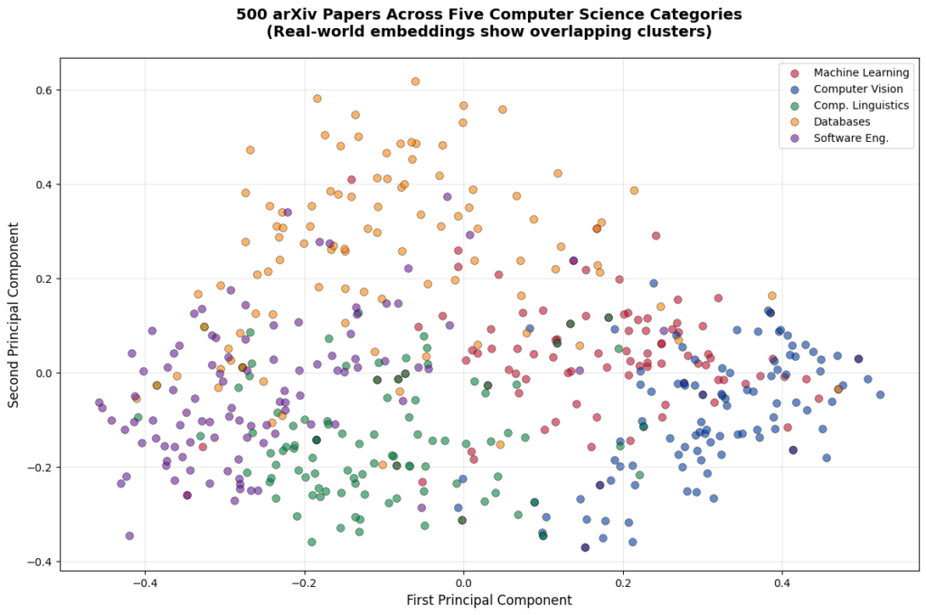
The visualization above reveals an important aspect of real-world data. Unlike our handcrafted examples in the previous tutorial, where clusters were perfectly separated, these real arXiv papers show more overlap. You can see clear groupings, as well as papers that bridge multiple topics. For example, a paper about "deep learning for database query optimization" uses vocabulary from both machine learning and databases, so it might appear between those clusters.

This is exactly what you'll encounter in production systems. Real data is messy, topics overlap, and semantic boundaries are often fuzzy rather than sharp. The embeddings are still capturing meaningful relationships, but the visualization shows the complexity of actual research papers rather than the idealized examples we used for learning.

Strategy Two: API-Based Embedding Services

Local models work great, but they require computational resources and you're responsible for managing them. API-based embedding services offer an alternative approach. You send your text to a cloud provider, they generate embeddings using their infrastructure, and they send the embeddings back to you.

We'll use Cohere's API for our main example because they offer a generous free trial tier that doesn't require payment information. This makes it perfect for learning and experimentation.

Setting Up Cohere Securely

First, you'll need to create a free Cohere account and get an API key:

1. Visit Cohere's registration page
2. Sign up for a free account (no credit card required)
3. Navigate to the API Keys section in your dashboard
4. Copy your Trial API key

Important security practice: Never hardcode API keys directly in your notebooks or scripts. Store them in a .env file instead. This prevents accidentally sharing sensitive credentials when you share your code.

Create a file named .env in your project directory with the following entry:

COHERE_API_KEY=your_key_here

Important: Add .env to your .gitignore file to prevent committing it to version control.

Now load your API key securely:

from dotenv import load_dotenv
import os
import cohere
import time

# Load environment variables from .env file
load_dotenv()

# Access your API key
cohere_api_key = os.getenv('COHERE_API_KEY')

if not cohere_api_key:
    raise ValueError(
        "COHERE_API_KEY not found. Please create a .env file with your API key.\n"
        "See https://dashboard.cohere.com for instructions on getting your key."
    )

# Initialize the Cohere client
co = cohere.Client(api_key=cohere_api_key)
print("API key loaded successfully from environment")

API key loaded successfully from environment

Now let's generate embeddings using the Cohere API. Here's something we discovered through trial and error: when we first ran this code without delays, we hit Cohere's rate limit and got a 429 TooManyRequestsError with this message: "trial token rate limit exceeded, limit is 100000 tokens per minute."

This exposes an important lesson about working with APIs. Rate limits aren't always clearly documented upfront. Sometimes you discover them by running into them, then you have to dig through the error responses in the documentation to understand what happened. In this case, we found the details in Cohere's error responses documentation. You can also check their rate limits page for current limits, though specifics for free tier accounts aren't always listed there.

With 500 papers averaging around 1,337 characters each, we can easily exceed 100,000 tokens per minute if we send batches too quickly. So we've built in two safeguards: a 12-second delay between batches to stay under the limit, and retry logic in case we do hit it. This makes the process take about 60-70 seconds instead of the 6-8 seconds the API actually needs, but it's reliable and won't throw errors mid-process.

Think of it as the tradeoff for using a free tier: we get access to powerful models without paying, but we work within some constraints. Let's see it in action:

print("Generating embeddings using Cohere API...")
print(f"Processing {len(abstracts)} abstracts...")

start_time = time.time()
actual_api_time = 0  # Track time spent on actual API calls

# Cohere recommends processing in batches for efficiency
# Their API accepts up to 96 texts per request
batch_size = 90
all_embeddings = []

for i in range(0, len(abstracts), batch_size):
    batch = abstracts[i:i+batch_size]
    batch_num = i//batch_size + 1
    total_batches = (len(abstracts) + batch_size - 1) // batch_size
    print(f"Processing batch {batch_num}/{total_batches} ({len(batch)} abstracts)...")

    # Add retry logic for rate limits
    max_retries = 3
    retry_delay = 60  # Wait 60 seconds if we hit rate limit

    for attempt in range(max_retries):
        try:
            # Track actual API call time
            api_start = time.time()

            # Generate embeddings for this batch
            response = co.embed(
                texts=batch,
                model='embed-english-v3.0',
                input_type='search_document'
            )

            actual_api_time += time.time() - api_start
            all_embeddings.extend(response.embeddings)
            break  # Success, move to next batch

        except Exception as e:
            if "rate limit" in str(e).lower() and attempt < max_retries - 1:
                print(f"  Rate limit hit. Waiting {retry_delay} seconds before retry...")
                time.sleep(retry_delay)
            else:
                raise  # Re-raise if it's not a rate limit error or we're out of retries

    # Add a delay between batches to avoid hitting rate limits
    # Wait 12 seconds between batches (spreads 500 papers over ~1 minute)
    if i + batch_size < len(abstracts):  # Don't wait after the last batch
        time.sleep(12)

# Convert to numpy array for consistency with local models
embeddings_cohere = np.array(all_embeddings)
elapsed_time = time.time() - start_time

print(f"\nCompleted in {elapsed_time:.2f} seconds (includes rate limit delays)")
print(f"Actual API processing time: {actual_api_time:.2f} seconds")
print(f"Time spent waiting for rate limits: {elapsed_time - actual_api_time:.2f} seconds")
print(f"Embedding shape: {embeddings_cohere.shape}")
print(f"Each abstract is now a {embeddings_cohere.shape[1]}-dimensional vector")
print(f"Average time per abstract (API only): {actual_api_time/len(abstracts):.3f} seconds")

# Add to DataFrame
df['embedding_cohere'] = list(embeddings_cohere)

Generating embeddings using Cohere API...
Processing 500 abstracts...
Processing batch 1/6 (90 abstracts)...
Processing batch 2/6 (90 abstracts)...
Processing batch 3/6 (90 abstracts)...
Processing batch 4/6 (90 abstracts)...
Processing batch 5/6 (90 abstracts)...
Processing batch 6/6 (50 abstracts)...

Completed in 66.31 seconds (includes rate limit delays)
Actual API processing time: 6.26 seconds
Time spent waiting for rate limits: 60.05 seconds
Embedding shape: (500, 1024)
Each abstract is now a 1024-dimensional vector
Average time per abstract (API only): 0.013 seconds

Notice the timing breakdown? The actual API processing was quite fast (around 6 seconds), but we spent most of our time waiting between batches to respect rate limits. This is the reality of free-tier accounts: they're fantastic for learning and prototyping, but come with constraints. Paid tiers would give us much higher limits and let us process at full speed.

For this tutorial, the free tier works perfectly. We're focusing on understanding the concepts and comparing approaches, not optimizing for production speed. The key differences from local models:

• No local computation: All processing happens on Cohere's servers, so it works equally well on any hardware.
• Internet dependency: Requires an active internet connection to work.
• Rate limits: Free tier accounts have token-per-minute limits, which is why we added delays between batches.

Other API Options

While we're using Cohere for this tutorial, you should know about other popular embedding APIs:

OpenAI offers excellent embedding models, but requires payment information upfront. If you have an OpenAI account, their text-embedding-3-small model is very affordable at \$0.02 per 1M tokens. You can find setup instructions in their embeddings documentation.

Together AI provides access to many open-source models through their API. They currently offer \$5 in free credits for new users. They offer models like BAAI/bge-large-en-v1.5 and detailed documentation at their embeddings guide. Note that free tier offerings change frequently, so check their current pricing when you sign up.

The choice between these services depends on your priorities. OpenAI has excellent quality but requires payment setup. Together AI offers many model choices with some free credits. Cohere has a truly free tier for learning and prototyping.

Comparing Your Options

Now that we've generated embeddings using both local models and an API service, let's think about how to choose between these approaches for real projects. The decision isn't about one being universally better than the other. It's about matching the approach to your specific constraints and requirements.

To clarify terminology: "self-hosted models" means running models on infrastructure you control, whether that's your laptop for learning or your company's cloud servers for production. "API services" means using third-party providers like Cohere or OpenAI where you send data to their servers for processing.

Dimension	Self-hosted Models	API Services
Cost	Zero ongoing costs after initial setup. Best for high-volume applications where you'll generate embeddings frequently.	Pay-per-use model per 1M tokens. Cohere: \$0.12 per 1M tokens. OpenAI: \$0.13 per 1M tokens. Best for low to moderate volume, or when you want predictable costs without infrastructure.
Performance	Speed depends on your hardware. Our results: 0.131 seconds per abstract (small model), 1.361 seconds per abstract (large model). Best for batch processing or when you control the infrastructure.	Speed depends on internet connection and API server load. Our results: 0.013 seconds per abstract (Cohere). Includes network latency and third-party infrastructure considerations. Best when you don't have powerful local hardware or need access to the latest models.
Privacy	All data stays on your infrastructure. Complete control over data handling. No data sent to third parties. Best for sensitive data, healthcare, financial services, or when compliance requires data locality.	Data is sent to third-party servers for processing. Subject to the provider's data handling policies. Cohere states that API data isn't used for training (verify current policy). Best for non-sensitive data, or when provider policies meet your requirements.
Customization	Can fine-tune models on your specific domain. Full control over model selection and updates. Can modify inference parameters. Best for specialized domains, custom requirements, or when you need reproducibility.	Limited to provider's available models. Model updates happen on provider's schedule. Less control over inference details. Best for general-purpose applications, or when using the latest models matters more than control.
Infrastructure	Requires managing infrastructure. Whether running on your laptop or company cloud servers, you handle model updates, dependencies, and scaling. Best for organizations with existing ML infrastructure or when infrastructure control is important.	No infrastructure management needed. Automatic scaling to handle load. Provider manages updates and availability. Best for smaller teams, rapid prototyping, or when you want to focus on application logic rather than infrastructure.

When to Use Each Approach

Here's a practical decision guide to help you choose the right approach for your project:

Choose Self-Hosted Models when you:

• Process large volumes of text regularly
• Work with sensitive or regulated data
• Need offline capability
• Have existing ML infrastructure (whether local or cloud-based)
• Want to fine-tune models for your domain
• Need complete control over the deployment

Choose API Services when you:

• Are just getting started or prototyping
• Have unpredictable or variable workload
• Want to avoid infrastructure management
• Need automatic scaling
• Prefer the latest models without maintenance
• Value simplicity over infrastructure control

For our tutorial series, we've used both approaches to give you hands-on experience with each. In our next tutorial, we'll use the Cohere embeddings for our semantic search implementation. We're choosing Cohere because they offer a generous free tier for learning (no payment required), their models are well-suited for semantic search tasks, and they work consistently across different hardware setups.

In practice, you'd evaluate embedding quality by testing on your specific use case: generate embeddings with different models, run similarity searches on sample queries, and measure which model returns the most relevant results for your domain.

Storing Your Embeddings

We've generated embeddings using multiple methods, and now we need to save them for future use. Storing embeddings properly is important because generating them can be time-consuming and potentially costly. You don't want to regenerate embeddings every time you run your code.

Let's explore two storage approaches:

Option 1: CSV with Numpy Arrays

This approach works well for learning and small-scale prototyping:

# Save the metadata to CSV (without embeddings, which are large arrays)
df_metadata = df[['title', 'abstract', 'authors', 'published', 'category', 'arxiv_id', 'abstract_length']]
df_metadata.to_csv('arxiv_papers_metadata.csv', index=False)
print("Saved metadata to 'arxiv_papers_metadata.csv'")

# Save embeddings as numpy arrays
np.save('embeddings_minilm.npy', embeddings_small)
np.save('embeddings_mpnet.npy', embeddings_large)
np.save('embeddings_cohere.npy', embeddings_cohere)
print("Saved embeddings to .npy files")

# Later, you can load them back like this:
# df_loaded = pd.read_csv('arxiv_papers_metadata.csv')
# embeddings_loaded = np.load('embeddings_cohere.npy')

Saved metadata to 'arxiv_papers_metadata.csv'
Saved embeddings to .npy files

This approach is simple and transparent, making it perfect for learning and experimentation. However, it has significant limitations for larger datasets:

• Loading all embeddings into memory doesn't scale beyond a few thousand documents
• No indexing for fast similarity search
• Manual coordination between CSV metadata and numpy arrays

For production systems with thousands or millions of embeddings, you'll want specialized vector databases (Option 2) that handle indexing, similarity search, and efficient storage automatically.

Option 2: Preparing for Vector Databases

In production systems, you'll likely store embeddings in a specialized vector database like Pinecone, Weaviate, or Chroma. These databases are optimized for similarity search. While we'll cover vector databases in detail in another tutorial series, here's how you'd structure your data for them:

# Prepare data in a format suitable for vector databases
# Most vector databases want: ID, embedding vector, and metadata

vector_db_data = []
for idx, row in df.iterrows():
    vector_db_data.append({
        'id': row['arxiv_id'],
        'embedding': row['embedding_cohere'].tolist(),  # Convert numpy array to list
        'metadata': {
            'title': row['title'],
            'abstract': row['abstract'][:500],  # Many DBs limit metadata size
            'authors': ', '.join(row['authors'][:3]),  # First 3 authors
            'category': row['category'],
            'published': str(row['published'])
        }
    })

# Save in JSON format for easy loading into vector databases
import json
with open('arxiv_papers_vector_db_format.json', 'w') as f:
    json.dump(vector_db_data, f, indent=2)
print("Saved data in vector database format to 'arxiv_papers_vector_db_format.json'")

print(f"\nTotal storage sizes:")
print(f"  Metadata CSV: ~{os.path.getsize('arxiv_papers_metadata.csv')/1024:.1f} KB")
print(f"  JSON for vector DB: ~{os.path.getsize('arxiv_papers_vector_db_format.json')/1024:.1f} KB")

Saved data in vector database format to 'arxiv_papers_vector_db_format.json'

Total storage sizes:
  Metadata CSV: ~773.2 KB
  JSON for vector DB: ~10137.3 KB

Each storage method has its purpose:

• CSV + numpy: Best for learning and small-scale experimentation
• JSON for vector databases: Best for production systems that need efficient similarity search

Preparing for Semantic Search

You now have 500 research papers from five distinct computer science domains with embeddings that capture their semantic meaning. These embeddings are vectors, which means we can measure how similar or different they are using mathematical distance calculations.

In the next tutorial, you'll use these embeddings to build a search system that finds relevant papers based on meaning rather than keywords. You'll implement similarity calculations, rank results, and see firsthand how semantic search outperforms traditional keyword matching.

Save your embeddings now, especially the Cohere embeddings since we'll use those in the next tutorial to build our search system. We chose Cohere because they work consistently across different hardware setups and provide a consistent baseline for implementing similarity calculations.

Next Steps

Before we move on, try these experiments to deepen your understanding:

Experiment with different arXiv categories:

• Try collecting papers from categories like stat.ML (Statistics Machine Learning) or math.OC (Optimization and Control)
• Use the PCA visualization code to see how these new categories cluster with your existing five
• Do some categories overlap more than others?

Compare embedding models visually:

• Generate embeddings for your dataset using all-mpnet-base-v2
• Create side-by-side PCA visualizations comparing the small model and large model
• Do the clusters look tighter or more separated with the larger model?

Test different dataset sizes:

• Collect just 50 papers per category (250 total) and visualize the results
• Then try 200 papers per category (1000 total)
• How does dataset size affect the clarity of the clusters?
• At what point does collection or processing time become noticeable?

Explore model differences:

• Visit Hugging Face's sentence similarity models
• Try a domain-specific model optimized for scientific text
• Compare the embeddings qualitatively by looking at which papers cluster together

These experiments will prepare you for the project that follows this tutorial series, where you'll apply these same techniques to build a Kaggle dataset search engine.

Ready to implement similarity search and build a working semantic search engine? The next tutorial will show you how to turn these embeddings into a powerful research discovery tool.

---

Key Takeaways:

• Programmatic data collection through APIs like arXiv enables working with real-world datasets
• Collecting papers from diverse categories (cs.LG, cs.CV, cs.CL, cs.DB, cs.SE) creates semantic clusters for effective search
• Papers can be cross-listed in multiple arXiv categories, creating natural overlap between related fields
• Self-hosted embedding models provide zero-cost, private embedding generation with full control over the process
• API-based embedding services offer high-quality embeddings without infrastructure management
• Secure credential handling using .env files protects sensitive API keys and tokens
• Rate limits aren't always clearly documented and are sometimes discovered through trial and error
• The choice between self-hosted and API approaches depends on cost, privacy, scale, and infrastructure considerations
• Free tier APIs provide powerful embedding generation for learning, but require handling rate limits and delays that paid tiers avoid
• Real-world embeddings show more overlap than handcrafted examples, reflecting the complexity of actual data
• Proper storage of embeddings prevents costly regeneration and enables efficient reuse across projects