An Uncomplicated Guide to Unsupervised Machine Learning
When starting out in machine learning, it's common to spend some time working to predict values. These values might be whether or not a credit card transaction is fraudulent, how much a customer earns based on their behavior patterns, etc. In scenarios like these, we're working with supervised machine learning.
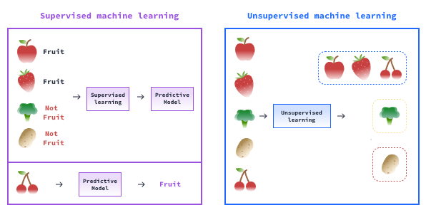
In supervised machine learning, the dataset contains a target variable that we're trying to predict. As the name suggests, we can supervise our model's performance since it's possible to objectively verify if its outputs are correct.
When working with unsupervised algorithms, we have an unlabelled dataset, which means we do not have a target variable that we'll try to predict. In fact, the goal is not to predict anything but, rather, to find patterns in the data.
Because there's no target variable, we can't supervise the algorithm by objectively determining whether or not the outputs are correct. Therefore, it's up to the data scientist to analyze the outputs and understand the pattern the algorithm found in the data.
The following diagram illustrates this difference:
The most common unsupervised machine learning types include the following:
* Clustering: the process of segmenting the dataset into groups based on the patterns found in the data — used to segment customers and products, for example.
-
Association: the goal is to find patterns between the variables, not the entries — frequently used for market basket analysis, for instance.
-
Anomaly detection: this kind of algorithm tries to identify when a particular data point is entirely off the rest of the dataset pattern — frequently used for fraud detection.
Clustering
Clustering algorithms segment a dataset into multiple groups based on the characteristics of each data point.
For instance, let's say we have a database containing data about thousands of customers. We could use clustering to segment these customers into categories in order to apply different marketing strategies for each group.
KMeans Algorithm
The K-means algorithm is an iterative algorithm designed to find a split for a dataset given a number of clusters set by the user. The number of clusters is called K.
In K-means, the algorithm randomly chooses K points to be the centers of the clusters. These points are called the clusters' centroids. K is set by the user. Then, an iterative process begins wherein each iteration is the process of assigning the data points to the closest centroid and recalculating the centroid as the mean of the points in the cluster. This process goes on and on until each centroid is located in the mean of its cluster.
The image below illustrates this process:

Now let's see an example of the K-means algorithm at work. We have a dataset of customers, and we're going to segment these customers based on their annual income and spending score. Here's how a plot representing these two variables looks:
import pandas as pd
import matplotlib.pyplot as plt
import seaborn as sns

# Reading the data
sns.set_style('whitegrid')
df = pd.read_csv('mall_customers.csv')

# Plotting the data
fig, ax = plt.subplots(figsize=(12, 6))

sns.scatterplot('Annual Income', 'Spending Score', data=df, ax=ax)

plt.tight_layout()
plt.show()
/usr/local/lib/python3.7/dist-packages/seaborn/_decorators.py:43: FutureWarning: Pass the following variables as keyword args: x, y. From version 0.12, the only valid positional argument will be <code>data</code>, and passing other arguments without an explicit keyword will result in an error or misinterpretation.
FutureWarning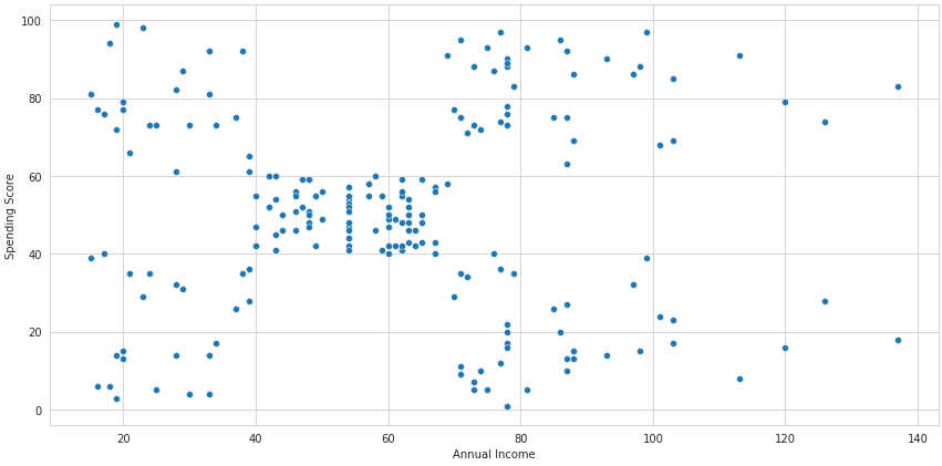
We'll then split the dataset into five clusters:
# Using KMeans
from sklearn.cluster import KMeans

model = KMeans(n_clusters=5)
y = model.fit_predict(df[['Annual Income', 'Spending Score']])

df['CLUSTER'] = y
Now we have the same plot grouped by the clusters we just created:
# Plotting the clustered data
fig, ax = plt.subplots(figsize=(12, 6))

sns.scatterplot('Annual Income', 'Spending Score', data=df, hue='CLUSTER', ax=ax, cmap='tab10')

plt.tight_layout()
plt.show()
/usr/local/lib/python3.7/dist-packages/seaborn/_decorators.py:43: FutureWarning: Pass the following variables as keyword args: x, y. From version 0.12, the only valid positional argument will be <code>data</code>, and passing other arguments without an explicit keyword will result in an error or misinterpretation.
FutureWarning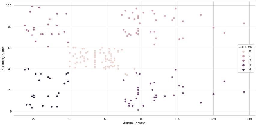
You can check KMeans documentation here.
Hierarchical Clustering
Hierarchical clustering is a clustering technique based on building a hierarchy between the clusters. This technique is subdivided into two main approaches:
- Agglomerative clustering
- Divisive clustering
The agglomeration, or bottoms-up, approach consists of assigning every data point as a single cluster and then going through an iterative process to group these clusters together.
Let's say, for instance, we have a 100-row dataset. At first, the bottoms-up approach will have 100 clusters. Then, each point is grouped to the closest one, creating larger clusters. These new clusters keep being grouped together with the closest ones until we have a single cluster containing all the points.
The divisive, or top-down, approach works in the opposite way. At first, all the data points are grouped into one cluster. Then the farthest point is taken out of the main cluster over and over until each point becomes its own cluster.
The bottoms-up approach is far more common than the top-down one, so let's see an example of its use. We're using a sample of the same dataset used in the K-means example. The image below is called a dendrogram, and it's how we visualize hierarchical clustering:
# Creating a dendogram with scipy
import scipy.cluster.hierarchy as shc

sample = df.sample(30)
plt.figure(figsize=(12,6))
dend = shc.dendrogram(shc.linkage(sample[['Annual Income', 'Spending Score']], method='ward'))
plt.grid(False)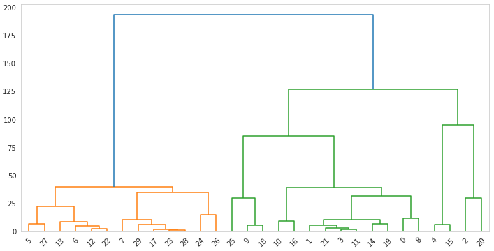
Notice that every single point is a cluster at the beginning, and then they are grouped until there's a single cluster.
Also, we've set the method as Ward. This is a common way of performing hierarchical clustering. This method makes the merge of clusters at each step of the clustering process by calculating on the sum of the square distances between the clusters. There are multiple other methods for this that use the maximum, minimum, and average distance — and more. You can check them all in the documentation.
We now need to set a cutoff point. There's no correct way of doing this, and deciding the number of clusters is probably the trickiest step of any clustering process. Several tools are useful to help you determine this number, such as the Silhouette and Elbow methods. In our case, we are creating two clusters and would have the dendrogram cut like this:
import scipy.cluster.hierarchy as shc

plt.figure(figsize=(12,6))
dend = shc.dendrogram(shc.linkage(sample[['Annual Income', 'Spending Score']], method='ward'))
plt.axhline(y=150, color='black', linestyle='--')

plt.grid(False)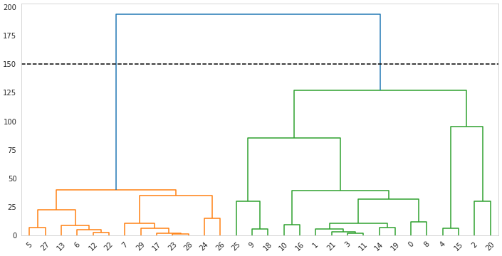
And from the cutoff point below, we are left with two clusters.
Association
Association is an unsupervised learning technique used to find "hidden" rules and patterns in data. Its classical use case is known as the market basket analysis.
The market basket analysis consists of discovering items that are highly correlated with each other. In other words, we use data from numerous purchases to determine which items are frequently bought together in order to make recommendations to customers in an online store, or to determine the best way to display products in a physical store.
We have a dataset containing information about thousands of purchases at a grocery store. In each row, we have an item that is part of a purchase. Here's how it looks:
# Reading the initial data
df = pd.read_csv('Groceries data.csv')
df.sort_values(['Member_number', 'Date']).head()| Member_number | Date | itemDescription | year | month | day | day_of_week | |
|---|---|---|---|---|---|---|---|
| 13331 | 1000 | 2014-06-24 | whole milk | 2014 | 6 | 24 | 1 |
| 29480 | 1000 | 2014-06-24 | pastry | 2014 | 6 | 24 | 1 |
| 32851 | 1000 | 2014-06-24 | salty snack | 2014 | 6 | 24 | 1 |
| 4843 | 1000 | 2015-03-15 | sausage | 2015 | 3 | 15 | 6 |
| 8395 | 1000 | 2015-03-15 | whole milk | 2015 | 3 | 15 | 6 |
  <script>
    const buttonEl =
      document.querySelector('#df-3742023f-1fd4-4dec-9942-de92e72af7f1 button.colab-df-convert');
    buttonEl.style.display =
      google.colab.kernel.accessAllowed ? 'block' : 'none';

    async function convertToInteractive(key) {
      const element = document.querySelector('#df-3742023f-1fd4-4dec-9942-de92e72af7f1');
      const dataTable =
        await google.colab.kernel.invokeFunction('convertToInteractive',
                                                 [key], {});
      if (!dataTable) return;

      const docLinkHtml = 'Like what you see? Visit the ' +
        '<a target="_blank" href=https://colab.research.google.com/notebooks/data_table.ipynb>data table notebook</a>'
        + ' to learn more about interactive tables.';
      element.innerHTML = '';
      dataTable['output_type'] = 'display_data';
      await google.colab.output.renderOutput(dataTable, element);
      const docLink = document.createElement('div');
      docLink.innerHTML = docLinkHtml;
      element.appendChild(docLink);
    }
  </script>
</div>
The first three rows are items purchased by the same client on the same day. We'll assume this is a single transaction.
We then manipulate this dataset in such a way (which is not the focus here) that every row becomes an entire transaction. We have a column for every unique item in the dataset deemed as True or False, depending on whether or not it's part of the transaction represented in that row:
# Reading data after manipulation
transactions = pd.read_csv('transactions.csv')
transactions = transactions.astype(bool)
transactions.head()| Instant food products | UHT-milk | abrasive cleaner | artif. sweetener | baby cosmetics | bags | baking powder | bathroom cleaner | beef | berries | ... | turkey | vinegar | waffles | whipped/sour cream | whisky | white bread | white wine | whole milk | yogurt | zwieback | |
|---|---|---|---|---|---|---|---|---|---|---|---|---|---|---|---|---|---|---|---|---|---|
| 0 | True | False | False | False | False | False | False | False | False | False | ... | False | False | False | True | False | False | False | False | False | False |
| 1 | True | False | False | False | False | False | False | False | False | False | ... | False | False | False | False | False | False | False | False | False | False |
| 2 | True | False | False | False | False | False | False | False | False | False | ... | False | False | False | False | False | False | False | False | False | False |
| 3 | True | False | False | False | False | False | False | False | False | False | ... | False | False | False | False | False | False | False | True | False | False |
| 4 | True | False | False | False | False | False | False | False | False | False | ... | False | False | False | False | False | False | False | False | False | False |
5 rows × 167 columns
  <script>
    const buttonEl =
      document.querySelector('#df-15b1938f-6f76-4e61-95a8-a57399fa2049 button.colab-df-convert');
    buttonEl.style.display =
      google.colab.kernel.accessAllowed ? 'block' : 'none';

    async function convertToInteractive(key) {
      const element = document.querySelector('#df-15b1938f-6f76-4e61-95a8-a57399fa2049');
      const dataTable =
        await google.colab.kernel.invokeFunction('convertToInteractive',
                                                 [key], {});
      if (!dataTable) return;

      const docLinkHtml = 'Like what you see? Visit the ' +
        '<a target="_blank" href=https://colab.research.google.com/notebooks/data_table.ipynb>data table notebook</a>'
        + ' to learn more about interactive tables.';
      element.innerHTML = '';
      dataTable['output_type'] = 'display_data';
      await google.colab.output.renderOutput(dataTable, element);
      const docLink = document.createElement('div');
      docLink.innerHTML = docLinkHtml;
      element.appendChild(docLink);
    }
  </script>
</div>
You can access this modified dataset here.
With this data, we'll then use the apriori algorithm. This is a famous algorithm used to identify sets of items that frequently appear together in a market basket, for instance. These sets go from one item to as many as we set. In our case, we don't want sets with more than three items:
# Using the apriori algorithm
from mlxtend.frequent_patterns import apriori

frequent_itemsets = apriori(transactions, min_support=0.001, use_colnames=True, max_len=3)
frequent_itemsets| support | itemsets | |
|---|---|---|
| 0 | 0.028612 | (Instant food products) |
| 1 | 0.016691 | (UHT-milk) |
| 2 | 0.001431 | (abrasive cleaner) |
| 3 | 0.001431 | (artif. sweetener) |
| 4 | 0.008107 | (baking powder) |
| ... | ... | ... |
| 1899 | 0.001431 | (whole milk, sausage, zwieback) |
| 1900 | 0.001431 | (soda, yogurt, tropical fruit) |
| 1901 | 0.001431 | (specialty chocolate, whole milk, yogurt) |
| 1902 | 0.001431 | (whipped/sour cream, yogurt, tropical fruit) |
| 1903 | 0.001907 | (whole milk, yogurt, tropical fruit) |
1904 rows × 2 columns
  <script>
    const buttonEl =
      document.querySelector('#df-cde9d389-b22c-4469-a724-c593d55841eb button.colab-df-convert');
    buttonEl.style.display =
      google.colab.kernel.accessAllowed ? 'block' : 'none';

    async function convertToInteractive(key) {
      const element = document.querySelector('#df-cde9d389-b22c-4469-a724-c593d55841eb');
      const dataTable =
        await google.colab.kernel.invokeFunction('convertToInteractive',
                                                 [key], {});
      if (!dataTable) return;

      const docLinkHtml = 'Like what you see? Visit the ' +
        '<a target="_blank" href=https://colab.research.google.com/notebooks/data_table.ipynb>data table notebook</a>'
        + ' to learn more about interactive tables.';
      element.innerHTML = '';
      dataTable['output_type'] = 'display_data';
      await google.colab.output.renderOutput(dataTable, element);
      const docLink = document.createElement('div');
      docLink.innerHTML = docLinkHtml;
      element.appendChild(docLink);
    }
  </script>
</div>
The support metric we see corresponds to the probability of that particular item set occurring. For instance, let's say we have a 100-basket dataset, in which the combination of milk and coffee occurs in 20 baskets. That means that this combination happens in 20% of baskets; therefore, the support is 0.20.
We'll now use a function to find rules in this data. This function will go over the sets created by the apriori algorithm in order to identify the products that are frequently bought together, and determine whether or not they are in the same set.
# Using association rules
from mlxtend.frequent_patterns import association_rules

rules = association_rules(frequent_itemsets, metric="lift",  min_threshold=1.5)

display(rules.head())
print(f"Number of rules: {len(rules)}")| antecedents | consequents | antecedent support | consequent support | support | confidence | lift | leverage | conviction | |
|---|---|---|---|---|---|---|---|---|---|
| 0 | (bottled beer) | (UHT-milk) | 0.041965 | 0.016691 | 0.001907 | 0.045455 | 2.723377 | 0.001207 | 1.030134 |
| 1 | (UHT-milk) | (bottled beer) | 0.016691 | 0.041965 | 0.001907 | 0.114286 | 2.723377 | 0.001207 | 1.081653 |
| 2 | (frankfurter) | (UHT-milk) | 0.031950 | 0.016691 | 0.001431 | 0.044776 | 2.682729 | 0.000897 | 1.029402 |
| 3 | (UHT-milk) | (frankfurter) | 0.016691 | 0.031950 | 0.001431 | 0.085714 | 2.682729 | 0.000897 | 1.058804 |
| 4 | (margarine) | (UHT-milk) | 0.032427 | 0.016691 | 0.001431 | 0.044118 | 2.643277 | 0.000889 | 1.028693 |
  <script>
    const buttonEl =
      document.querySelector('#df-e167da81-504a-4fb4-a07e-f405d4ef9d8d button.colab-df-convert');
    buttonEl.style.display =
      google.colab.kernel.accessAllowed ? 'block' : 'none';

    async function convertToInteractive(key) {
      const element = document.querySelector('#df-e167da81-504a-4fb4-a07e-f405d4ef9d8d');
      const dataTable =
        await google.colab.kernel.invokeFunction('convertToInteractive',
                                                 [key], {});
      if (!dataTable) return;

      const docLinkHtml = 'Like what you see? Visit the ' +
        '<a target="_blank" href=https://colab.research.google.com/notebooks/data_table.ipynb>data table notebook</a>'
        + ' to learn more about interactive tables.';
      element.innerHTML = '';
      dataTable['output_type'] = 'display_data';
      await google.colab.output.renderOutput(dataTable, element);
      const docLink = document.createElement('div');
      docLink.innerHTML = docLinkHtml;
      element.appendChild(docLink);
    }
  </script>
</div>
Number of rules: 2388Other than the support, there are two other important metrics we should be aware of.
Confidence is the probability that a complete transaction will occur given that their first item is already in that basket. In other words, let's say the probability (support) of a person buying milk and also buying coffee is 0.5 and the probability (support) of a person buying just coffee is 0.10. The confidence is then 0.10 over 0.05 which is equal to 0.5. Putting it mathematically:
$$ confidence(milk→coffee) = \frac{support(milk→coffee)} {support(milk)} $$
The Lift metric represents how much more often the rule occurs than we should expect it to. If the lift is equal to 1, it means that the items are statistically independent of each other, and no rules can be drawn from them. Therefore, the higher the lift, the more confident we are in the rule. Notice that, in the code, we chose to rank our rules by the lift and set a minimum threshold of 1.5.
Mathematically, the lift is confidence over support of the second item:
$$ lift(milk→coffee) = \frac{confidence(milk→coffee)} {support(milk→coffee)} $$
The are also a few other metrics. Check the documentation to go over them all.
Anomaly Detection
Anomaly detection is the process of finding abnormal data points in a dataset. In other words, we're looking for outliers and points that are completely out of the dataset's patterns.
This kind of machine learning is commonly used to detect fraudulent credit card transactions or failures or imminent failures in a piece of equipment or machine.
Although we're dealing with anomaly detection as an unsupervised machine learning process, it can also be performed as a supervised algorithm. To do that, however, we'd need a labeled dataset for which we know whether or not each data point is an anomaly in order to train a model to carry on the classification task.
But we don't always have all the data we want. If we don't have that labeled dataset, then it becomes an unsupervised learning problem, and anomaly detection algorithms can help us.
When we talk about anomaly detection, we're not talking about a single kind of algorithm. There are multiple different algorithms used for this same task, and each of them uses different strategies and gets to different solutions.
Scikit-learn has a handful of different algorithms implemented for anomaly detection. Here, we'll offer a quick introduction and comparison between just three of them, but feel free to check the great Scikit-learn's documentation for more.
Isolation Forest
The Isolation Forest is a tree-based algorithm used for anomaly detection. The algorithm works by randomly selecting both a feature and a split value in this feature. This process goes on until we have the data points isolated as nodes in the tree.
The randomness of the process makes it so that an abnormal data point needs far fewer splits to be isolated than others. Because the entire tree is created multiple times, that's why we call it a "forest." When the same observation gets isolated quickly multiple times, the algorithm feels safe to assume it's an anomaly.
To create a quick example using Scikit-learn's implementation of Isolation Forest, we'll use the same customer's dataset as in the Clustering section, considering the same two variables: annual income, and spending score.
The following code uses the algorithm to create a new column in the dataset containing -1 for anomalies and 1 for non-anomalies. The scatter plot allows us to see how these classes are distributed:
# using the Isolation Forest algorithm
from sklearn.ensemble import IsolationForest

model = IsolationForest()
y_pred = model.fit_predict(df[['Annual Income', 'Spending Score']])
df['class'] = y_pred

# Plotting the data
fig, ax = plt.subplots(figsize=(12, 6))

sns.scatterplot('Annual Income', 'Spending Score', data=df, hue='class', ax=ax, cmap='tab10', alpha=0.8)

plt.tight_layout()
plt.show()
/usr/local/lib/python3.7/dist-packages/seaborn/_decorators.py:43: FutureWarning: Pass the following variables as keyword args: x, y. From version 0.12, the only valid positional argument will be <code>data</code>, and passing other arguments without an explicit keyword will result in an error or misinterpretation.
FutureWarning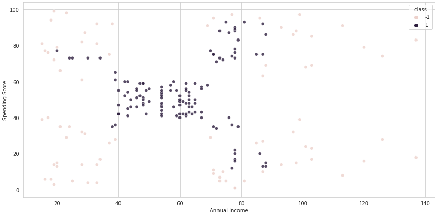
DBSCAN
DBSCAN is short for Density-Based Spatial Clustering of Applications with Noise. This is not only an anomaly detection algorithm but also a clustering algorithm. It works by segmenting the observations into three main classes.
The Base class is made by the observations that have a certain number of neighbors within a circle of a determined radius. The number of neighbors and the radius of the circle are hyperparameters to be set by the user.
The Border observations have less than the established number o neighbors but still have at least one, while the observations with no neighbors at all are considered of the Noise class.
The algorithm iteratively selects random points and, based on the hyperparameters, determines to which class they belong. This goes on until all the observations have been assigned to a class.
As mentioned, DBSCAN can produce multiple clusters since it's possible that we have Base observations farthest from each other than the radius hyperparameter.
Let's run DBSCAN in the same dataset as we ran the Isolation Forest. We'll set the radius equal to 12 and the number of neighbors equal to 5 as an example:
# Using DBSCAN
from sklearn.cluster import DBSCAN

model = DBSCAN(eps=12, min_samples=5)
y_pred = model.fit_predict(df[['Annual Income', 'Spending Score']])
df['class'] = y_pred

# Plotting the data
fig, ax = plt.subplots(figsize=(12, 6))

sns.scatterplot('Annual Income', 'Spending Score', data=df, hue='class', ax=ax, cmap='tab10')

plt.tight_layout()
plt.show()
/usr/local/lib/python3.7/dist-packages/seaborn/_decorators.py:43: FutureWarning: Pass the following variables as keyword args: x, y. From version 0.12, the only valid positional argument will be <code>data</code>, and passing other arguments without an explicit keyword will result in an error or misinterpretation.
FutureWarning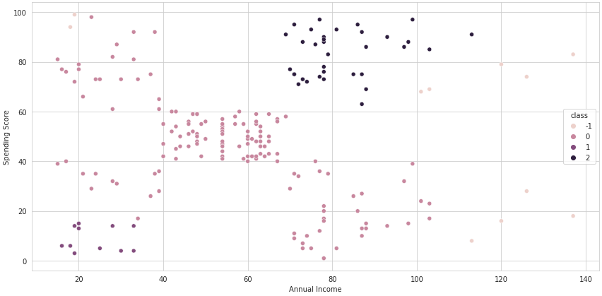
Notice that we have fewer anomalies than we had with Isolation Forest.
Local Outlier Factor
The Local Outlier Factor - LOF works similarly to the DBSCAN algorithm. They are both based on finding data points that do not belong to any local group of observations. The main difference is that the Local Outlier Factor issues another algorithm, K-nearest neighbors - KNN, to determine the local density.
The number K of is set by the user and is passed to KNN to determine the group of neighbors of each data point. When we compare the local density of one observation to the local density of its neighbors, it's possible to identify both regions of similar density and observation with significantly lower density than its neighbor, which is considered to be anomalies or outliers.
Using Scikit-learn's implementation and creating a scatter plot, we can see that the anomalies are not located only at the edges of the plot but distributed throughout the entire plot. That's because we're deciding whether or not they are anomalies based on their locality and distance from close neighbors.
# Usinsg Local Outlier Factor
from sklearn.neighbors import LocalOutlierFactor
model = LocalOutlierFactor(n_neighbors=2)
y_pred = model.fit_predict(df[['Annual Income', 'Spending Score']])
df['class'] = y_pred

# Plotting the data
fig, ax = plt.subplots(figsize=(12, 6))

sns.scatterplot('Annual Income', 'Spending Score', data=df, hue='class', ax=ax, cmap='tab10')

plt.tight_layout()
plt.show()
/usr/local/lib/python3.7/dist-packages/seaborn/_decorators.py:43: FutureWarning: Pass the following variables as keyword args: x, y. From version 0.12, the only valid positional argument will be <code>data</code>, and passing other arguments without an explicit keyword will result in an error or misinterpretation.
FutureWarning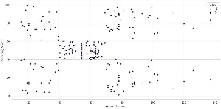
The different approaches for anomaly detection generated different outcomes from each other as we expected. The same would've happened if we had tested more algorithms. As mentioned earlier, each algorithm uses a different method to identify outliers and understanding these algorithms is crucial for achieving a better result.
Wrap Up & Next Steps
This article aimed to be a quick introduction to the usefulness and power of unsupervised machine learning. We explored the difference between supervised and unsupervised machine learning, and we also went through some important use cases, algorithms, and examples of unsupervised learning.
If you're interested in learning more about this subject, Dataquest's Data Scientist learning path is a great option to dive into both supervised and unsupervised machine learning. Make sure to check it out!