Measuring Similarity and Distance between Embeddings

In the previous tutorial, you learned how to collect 500 research papers from arXiv and generate embeddings using both local models and API services. You now have a dataset of papers with embeddings that capture their semantic meaning. Those embeddings are vectors, which means we can perform mathematical operations on them.

But here's the thing: having embeddings isn't enough to build a search system. You need to know how to measure similarity between vectors. When a user searches for "neural networks for computer vision," which papers in your dataset are most relevant? The answer lies in measuring the distance between the query embedding and each paper embedding.

This tutorial teaches you how to implement similarity calculations and build a functional semantic search engine. You'll implement three different distance metrics, understand when to use each one, and create a search function that returns ranked results based on semantic similarity. By the end, you'll have built a complete search system that finds relevant papers based on meaning rather than keywords.

Although this is the final tutorial in our series on embeddings, your learning doesn't need to stop here. We've designed a follow-up practice project where you can apply everything you've learned in this series to build a Kaggle dataset search engine. The practice project will demonstrate your ability to collect data, generate embeddings, and implement semantic search. This tutorial gives you the final missing piece for the project: implementing the search itself.

Setting Up Your Environment

We'll continue using the same libraries from the previous tutorials. If you've been following along, you should already have these installed. If not, here's the installation command for you to run from your terminal:

# Developed with: Python 3.12.12
# scikit-learn==1.6.1
# matplotlib==3.10.0
# numpy==2.0.2
# pandas==2.2.2
# cohere==5.20.0
# python-dotenv==1.1.1

pip install scikit-learn matplotlib numpy pandas cohere python-dotenv

Loading Your Saved Embeddings

Previously, we saved our embeddings and metadata to disk. Let's load them back into memory so we can work with them. We'll use the Cohere embeddings (embeddings_cohere.npy) because they provide consistent results across different hardware setups:

import numpy as np
import pandas as pd

# Load the metadata
df = pd.read_csv('arxiv_papers_metadata.csv')
print(f"Loaded {len(df)} papers")

# Load the Cohere embeddings
embeddings = np.load('embeddings_cohere.npy')
print(f"Loaded embeddings with shape: {embeddings.shape}")
print(f"Each paper is represented by a {embeddings.shape[1]}-dimensional vector")

# Verify the data loaded correctly
print(f"\nFirst paper title: {df['title'].iloc[0]}")
print(f"First embedding (first 5 values): {embeddings[0][:5]}")

Loaded 500 papers
Loaded embeddings with shape: (500, 1536)
Each paper is represented by a 1536-dimensional vector

First paper title: Dark Energy Survey Year 3 results: Simulation-based $w$CDM inference from weak lensing and galaxy clustering maps with deep learning. I. Analysis design
First embedding (first 5 values): [-7.7144260e-03  1.9527141e-02 -4.2141182e-05 -2.8627755e-03 -2.5192423e-02]

Perfect! We have our 500 papers and their corresponding 1536-dimensional embedding vectors. Each vector is a point in high-dimensional space, and papers with similar content will have vectors that are close together. Now we need to define what "close together" actually means.

Understanding Distance in Vector Space

Before we write any code, let's build intuition about measuring similarity between vectors. Imagine you have two papers about software compliance. Their embeddings might look like this:

Paper A: [0.8, 0.6, 0.1, ...]  (1536 numbers total)
Paper B: [0.7, 0.5, 0.2, ...]  (1536 numbers total)

To calculate the distance between embedding vectors, we need a distance metric. There are three commonly used metrics for measuring similarity between embeddings:

1. Euclidean Distance: Measures the straight-line distance between vectors in space. A shorter distance means higher similarity. You can think of it as measuring the physical distance between two points.
2. Dot Product: Multiplies corresponding elements and sums them up. Considers both direction and magnitude of the vectors. Works well when embeddings are normalized to unit length.
3. Cosine Similarity: Measures the angle between vectors. If two vectors point in the same direction, they're similar, regardless of their length. This is the most common metric for text embeddings.

We'll implement each metric in order from most intuitive to most commonly used. Let's start with Euclidean distance because it's the easiest to understand.

Implementing Euclidean Distance

Euclidean distance measures the straight-line distance between two points in space. This is the most intuitive metric because we all understand physical distance. If you have two points on a map, the Euclidean distance is literally how far apart they are.

Unlike the other metrics we'll learn (where higher is better), Euclidean distance works in reverse: lower distance means higher similarity. Papers that are close together in space have low distance and are semantically similar.

Note that Euclidean distance is sensitive to vector magnitude. If your embeddings aren't normalized (meaning vectors can have different lengths), two vectors pointing in similar directions but with different magnitudes will show larger distance than expected. This is why cosine similarity (which we'll learn next) is often preferred for text embeddings. It ignores magnitude and focuses purely on direction.

The formula is:

$$\text{Euclidean distance} = |\mathbf{A} - \mathbf{B}| = \sqrt{\sum_{i=1}^{n} (A_i - B_i)^2}$$

This is essentially the Pythagorean theorem extended to high-dimensional space. We subtract corresponding values, square them, sum everything up, and take the square root. Let's implement it:

def euclidean_distance_manual(vec1, vec2):
    """
    Calculate Euclidean distance between two vectors.

    Parameters:
    -----------
    vec1, vec2 : numpy arrays
        The vectors to compare

    Returns:
    --------
    float
        Euclidean distance (lower means more similar)
    """
    # np.linalg.norm computes the square root of sum of squared differences
    # This implements the Euclidean distance formula directly
    return np.linalg.norm(vec1 - vec2)

# Let's test it by comparing two similar papers
paper_idx_1 = 492  # Android compliance detection paper
paper_idx_2 = 493  # GDPR benchmarking paper

distance = euclidean_distance_manual(embeddings[paper_idx_1], embeddings[paper_idx_2])

print(f"Comparing two papers:")
print(f"Paper 1: {df['title'].iloc[paper_idx_1][:50]}...")
print(f"Paper 2: {df['title'].iloc[paper_idx_2][:50]}...")
print(f"\nEuclidean distance: {distance:.4f}")

Comparing two papers:
Paper 1: Can Large Language Models Detect Real-World Androi...
Paper 2: GDPR-Bench-Android: A Benchmark for Evaluating Aut...

Euclidean distance: 0.8431

A distance of 0.84 is quite low, which means these papers are very similar! Both papers discuss Android compliance and benchmarking, so this makes perfect sense. Now let's compare this to a paper from a completely different category:

# Compare a software engineering paper to a database paper
paper_idx_3 = 300  # A database paper about natural language queries

distance_related = euclidean_distance_manual(embeddings[paper_idx_1],
                                             embeddings[paper_idx_2])
distance_unrelated = euclidean_distance_manual(embeddings[paper_idx_1],
                                               embeddings[paper_idx_3])

print(f"Software Engineering paper 1 vs Software Engineering paper 2:")
print(f"  Distance: {distance_related:.4f}")
print(f"\nSoftware Engineering paper vs Database paper:")
print(f"  Distance: {distance_unrelated:.4f}")
print(f"\nThe related SE papers are {distance_unrelated/distance_related:.2f}x closer")

Software Engineering paper 1 vs Software Engineering paper 2:
  Distance: 0.8431

Software Engineering paper vs Database paper:
  Distance: 1.2538

The related SE papers are 1.49x closer

The distance correctly identifies that papers from the same category are closer to each other than papers from different categories. The related papers have a much lower distance.

For calculating distance to all papers, we can use scikit-learn:

from sklearn.metrics.pairwise import euclidean_distances

# Calculate distance from one paper to all others
query_embedding = embeddings[paper_idx_1].reshape(1, -1)
all_distances = euclidean_distances(query_embedding, embeddings)

# Get top 10 (lowest distances = most similar)
top_indices = np.argsort(all_distances[0])[1:11]

print(f"Query paper: {df['title'].iloc[paper_idx_1]}\n")
print("Top 10 papers by Euclidean distance (lowest = most similar):")
for rank, idx in enumerate(top_indices, 1):
    print(f"{rank}. [{all_distances[0][idx]:.4f}] {df['title'].iloc[idx][:50]}...")

Query paper: Can Large Language Models Detect Real-World Android Software Compliance Violations?

Top 10 papers by Euclidean distance (lowest = most similar):
1. [0.8431] GDPR-Bench-Android: A Benchmark for Evaluating Aut...
2. [1.0168] An Empirical Study of LLM-Based Code Clone Detecti...
3. [1.0218] LLM-as-a-Judge is Bad, Based on AI Attempting the ...
4. [1.0541] BengaliMoralBench: A Benchmark for Auditing Moral ...
5. [1.0677] Exploring the Feasibility of End-to-End Large Lang...
6. [1.0730] Where Do LLMs Still Struggle? An In-Depth Analysis...
7. [1.0730] Where Do LLMs Still Struggle? An In-Depth Analysis...
8. [1.0763] EvoDev: An Iterative Feature-Driven Framework for ...
9. [1.0766] Watermarking Large Language Models in Europe: Inte...
10. [1.0814] One Battle After Another: Probing LLMs' Limits on ...

Euclidean distance is intuitive and works well for many applications. Now let's learn about dot product, which takes a different approach to measuring similarity.

Implementing Dot Product Similarity

The dot product is simpler than Euclidean distance because it doesn't involve taking square roots or differences. Instead, we multiply corresponding elements and sum them up. The formula is:

$$\text{dot product} = \mathbf{A} \cdot \mathbf{B} = \sum_{i=1}^{n} A_i B_i$$

The dot product considers both the angle between vectors and their magnitudes. When vectors point in similar directions, the products of corresponding elements tend to be positive and large, resulting in a high dot product. When vectors point in different directions, some products are positive and some negative, and they tend to cancel out, resulting in a lower dot product. Higher scores mean higher similarity.

The dot product works particularly well when embeddings have been normalized to similar lengths. Many embedding APIs like Cohere and OpenAI produce normalized embeddings by default. However, some open-source frameworks (like sentence-transformers or instructor) require you to explicitly set normalization parameters. Always check your embedding model's documentation to understand whether normalization is applied automatically or needs to be configured.

Let's implement it:

def dot_product_similarity_manual(vec1, vec2):
    """
    Calculate dot product between two vectors.

    Parameters:
    -----------
    vec1, vec2 : numpy arrays
        The vectors to compare

    Returns:
    --------
    float
        Dot product score (higher means more similar)
    """
    # np.dot multiplies corresponding elements and sums them
    # This directly implements the dot product formula
    return np.dot(vec1, vec2)

# Compare the same papers using dot product
similarity_dot = dot_product_similarity_manual(embeddings[paper_idx_1],
                                               embeddings[paper_idx_2])

print(f"Comparing the same two papers:")
print(f"  Dot product: {similarity_dot:.4f}")

Comparing the same two papers:
  Dot product: 0.6446

Keep this number in mind. When we calculate cosine similarity next, you'll see why dot product works so well for these embeddings.

For search across all papers, we can use NumPy's matrix multiplication:

# Efficient dot product for one query against all papers
query_embedding = embeddings[paper_idx_1]
all_dot_products = np.dot(embeddings, query_embedding)

# Get top 10 results
top_indices = np.argsort(all_dot_products)[::-1][1:11]

print(f"Query paper: {df['title'].iloc[paper_idx_1]}\n")
print("Top 10 papers by dot product similarity:")
for rank, idx in enumerate(top_indices, 1):
    print(f"{rank}. [{all_dot_products[idx]:.4f}] {df['title'].iloc[idx][:50]}...")

Query paper: Can Large Language Models Detect Real-World Android Software Compliance Violations?

Top 10 papers by dot product similarity:
1. [0.6446] GDPR-Bench-Android: A Benchmark for Evaluating Aut...
2. [0.4831] An Empirical Study of LLM-Based Code Clone Detecti...
3. [0.4779] LLM-as-a-Judge is Bad, Based on AI Attempting the ...
4. [0.4445] BengaliMoralBench: A Benchmark for Auditing Moral ...
5. [0.4300] Exploring the Feasibility of End-to-End Large Lang...
6. [0.4243] Where Do LLMs Still Struggle? An In-Depth Analysis...
7. [0.4243] Where Do LLMs Still Struggle? An In-Depth Analysis...
8. [0.4208] EvoDev: An Iterative Feature-Driven Framework for ...
9. [0.4204] Watermarking Large Language Models in Europe: Inte...
10. [0.4153] One Battle After Another: Probing LLMs' Limits on ...

Notice that the rankings are identical to those from Euclidean distance! This happens because both metrics capture similar relationships in the data, just measured differently. This won't always be the case with all embedding models, but it's common when embeddings are well-normalized.

Implementing Cosine Similarity

Cosine similarity is the most commonly used metric for text embeddings. It measures the angle between vectors rather than their distance. If two vectors point in the same direction, they're similar, regardless of how long they are.

The formula looks like this:

$$\text{Cosine Similarity} = \frac{\mathbf{A} \cdot \mathbf{B}}{|\mathbf{A}| |\mathbf{B}|}=\frac{\sum_{i=1}^{n} A_i B_i}{\sqrt{\sum_{i=1}^{n} A_i^2} \sqrt{\sum_{i=1}^{n} B_i^2}}$$

Where $\mathbf{A}$ and $\mathbf{B}$ are our two vectors, $\mathbf{A} \cdot \mathbf{B}$ is the dot product, and $|\mathbf{A}|$ represents the magnitude (or length) of vector $\mathbf{A}$.

The result ranges from -1 to 1:

• 1 means the vectors point in exactly the same direction (identical meaning)
• 0 means the vectors are perpendicular (unrelated)
• -1 means the vectors point in opposite directions (opposite meaning)

For text embeddings, you'll typically see values between 0 and 1 because embeddings rarely point in completely opposite directions.

Let's implement this using NumPy:

def cosine_similarity_manual(vec1, vec2):
    """
    Calculate cosine similarity between two vectors.

    Parameters:
    -----------
    vec1, vec2 : numpy arrays
        The vectors to compare

    Returns:
    --------
    float
        Cosine similarity score between -1 and 1
    """
    # Calculate dot product (numerator)
    dot_product = np.dot(vec1, vec2)

    # Calculate magnitudes using np.linalg.norm (denominator)
    # np.linalg.norm computes sqrt(sum of squared values)
    magnitude1 = np.linalg.norm(vec1)
    magnitude2 = np.linalg.norm(vec2)

    # Divide dot product by product of magnitudes
    similarity = dot_product / (magnitude1 * magnitude2)

    return similarity

# Test with our software engineering papers
similarity = cosine_similarity_manual(embeddings[paper_idx_1],
                                     embeddings[paper_idx_2])

print(f"Comparing two papers:")
print(f"Paper 1: {df['title'].iloc[paper_idx_1][:50]}...")
print(f"Paper 2: {df['title'].iloc[paper_idx_2][:50]}...")
print(f"\nCosine similarity: {similarity:.4f}")

Comparing two papers:
Paper 1: Can Large Language Models Detect Real-World Androi...
Paper 2: GDPR-Bench-Android: A Benchmark for Evaluating Aut...

Cosine similarity: 0.6446

The cosine similarity (0.6446) is identical to the dot product we calculated earlier. This isn't a coincidence. Cohere's embeddings are normalized to unit length, which means the dot product and cosine similarity are mathematically equivalent for these vectors. When embeddings are normalized, the denominator in the cosine formula (the product of the vector magnitudes) always equals 1, leaving just the dot product. This is why many vector databases prefer dot product for normalized embeddings. It's computationally cheaper and produces identical results to cosine.

Now let's compare this to a paper from a completely different category:

# Compare a software engineering paper to a database paper
similarity_related = cosine_similarity_manual(embeddings[paper_idx_1],
                                             embeddings[paper_idx_2])
similarity_unrelated = cosine_similarity_manual(embeddings[paper_idx_1],
                                               embeddings[paper_idx_3])

print(f"Software Engineering paper 1 vs Software Engineering paper 2:")
print(f"  Similarity: {similarity_related:.4f}")
print(f"\nSoftware Engineering paper vs Database paper:")
print(f"  Similarity: {similarity_unrelated:.4f}")
print(f"\nThe SE papers are {similarity_related/similarity_unrelated:.2f}x more similar")

Software Engineering paper 1 vs Software Engineering paper 2:
  Similarity: 0.6446

Software Engineering paper vs Database paper:
  Similarity: 0.2140

The SE papers are 3.01x more similar

Great! The similarity score correctly identifies that papers from the same category are much more similar to each other than papers from different categories.

Now, calculating similarity one pair at a time is fine for understanding, but it's not practical for search. We need to compare a query against all 500 papers efficiently. Let's use scikit-learn's optimized implementation:

from sklearn.metrics.pairwise import cosine_similarity

# Calculate similarity between one paper and all other papers
query_embedding = embeddings[paper_idx_1].reshape(1, -1)
all_similarities = cosine_similarity(query_embedding, embeddings)

# Get the top 10 most similar papers (excluding the query itself)
top_indices = np.argsort(all_similarities[0])[::-1][1:11]

print(f"Query paper: {df['title'].iloc[paper_idx_1]}\n")
print("Top 10 most similar papers:")
for rank, idx in enumerate(top_indices, 1):
    print(f"{rank}. [{all_similarities[0][idx]:.4f}] {df['title'].iloc[idx][:50]}...")

Query paper: Can Large Language Models Detect Real-World Android Software Compliance Violations?

Top 10 most similar papers:
1. [0.6446] GDPR-Bench-Android: A Benchmark for Evaluating Aut...
2. [0.4831] An Empirical Study of LLM-Based Code Clone Detecti...
3. [0.4779] LLM-as-a-Judge is Bad, Based on AI Attempting the ...
4. [0.4445] BengaliMoralBench: A Benchmark for Auditing Moral ...
5. [0.4300] Exploring the Feasibility of End-to-End Large Lang...
6. [0.4243] Where Do LLMs Still Struggle? An In-Depth Analysis...
7. [0.4243] Where Do LLMs Still Struggle? An In-Depth Analysis...
8. [0.4208] EvoDev: An Iterative Feature-Driven Framework for ...
9. [0.4204] Watermarking Large Language Models in Europe: Inte...
10. [0.4153] One Battle After Another: Probing LLMs' Limits on ...

Notice how scikit-learn's cosine_similarity function is much cleaner. It handles the reshaping and broadcasts the calculation efficiently across all papers. This is what you'll use in production code, but understanding the manual implementation helps you see what's happening under the hood.

You might notice papers 6 and 7 appear to be duplicates with identical scores. This happens because the same paper was cross-listed in multiple arXiv categories. In a production system, you'd typically de-duplicate results using a stable identifier like the arXiv ID, showing each unique paper only once while perhaps noting all its categories.

Choosing the Right Metric for Your Use Case

Now that we've implemented all three metrics, let's understand when to use each one. Here's a practical comparison:

Metric	When to Use	Advantages	Considerations
Euclidean Distance	Use when the absolute position in vector space matters, or for scientific computing applications.	Intuitive geometric interpretation. Common in general machine learning tasks beyond NLP.	Lower scores mean higher similarity (inverse relationship). Can be sensitive to vector magnitude.
Dot Product	Use when embeddings are already normalized to unit length. Common in vector databases.	Fastest computation. Identical rankings to cosine for normalized vectors. Many vector DBs optimize for this.	Only equivalent to cosine when vectors are normalized. Check your embedding model's documentation.
Cosine Similarity	Default choice for text embeddings. Use when you care about semantic similarity regardless of document length.	Most common in NLP. Normalized by default (outputs 0 to 1). Works well with sentence-transformers and most embedding APIs.	Requires normalization calculation. Slightly more computationally expensive than dot product.

Going forward, we'll use cosine similarity because it's the standard for text embeddings and produces interpretable scores between 0 and 1.

Let's verify that our embeddings produce consistent rankings across metrics:

# Compare rankings from all three metrics for a single query
query_embedding = embeddings[paper_idx_1].reshape(1, -1)

# Calculate similarities/distances
cosine_scores = cosine_similarity(query_embedding, embeddings)[0]
dot_scores = np.dot(embeddings, embeddings[paper_idx_1])
euclidean_scores = euclidean_distances(query_embedding, embeddings)[0]

# Get top 10 indices for each metric
top_cosine = set(np.argsort(cosine_scores)[::-1][1:11])
top_dot = set(np.argsort(dot_scores)[::-1][1:11])
top_euclidean = set(np.argsort(euclidean_scores)[1:11])

# Calculate overlap
cosine_dot_overlap = len(top_cosine & top_dot)
cosine_euclidean_overlap = len(top_cosine & top_euclidean)
all_three_overlap = len(top_cosine & top_dot & top_euclidean)

print(f"Top 10 papers overlap between metrics:")
print(f"  Cosine & Dot Product: {cosine_dot_overlap}/10 papers match")
print(f"  Cosine & Euclidean: {cosine_euclidean_overlap}/10 papers match")
print(f"  All three metrics: {all_three_overlap}/10 papers match")

Top 10 papers overlap between metrics:
  Cosine & Dot Product: 10/10 papers match
  Cosine & Euclidean: 10/10 papers match
  All three metrics: 10/10 papers match

For our Cohere embeddings with these 500 papers, all three metrics produce identical top-10 rankings. This happens when embeddings are well-normalized, but isn't guaranteed across all embedding models or datasets. What matters more than perfect metric agreement is understanding what each metric measures and when to use it.

Building Your Search Function

Now let's build a complete semantic search function that ties everything together. This function will take a natural language query, convert it into an embedding, and return the most relevant papers.

Before building our search function, ensure your Cohere API key is configured. As we did in the previous tutorial, you should have a .env file in your project directory with your API key:

COHERE_API_KEY=your_key_here

Now let's build the search function:

from cohere import ClientV2
from dotenv import load_dotenv
import os

# Load Cohere API key
load_dotenv()
cohere_api_key = os.getenv('COHERE_API_KEY')
co = ClientV2(api_key=cohere_api_key)

def semantic_search(query, embeddings, df, top_k=5, metric='cosine'):
    """
    Search for papers semantically similar to a query.

    Parameters:
    -----------
    query : str
        Natural language search query
    embeddings : numpy array
        Pre-computed embeddings for all papers
    df : pandas DataFrame
        DataFrame containing paper metadata
    top_k : int
        Number of results to return
    metric : str
        Similarity metric to use ('cosine', 'dot', or 'euclidean')

    Returns:
    --------
    pandas DataFrame
        Top results with similarity scores
    """
    # Generate embedding for the query
    response = co.embed(
        texts=[query],
        model='embed-v4.0',
        input_type='search_query',
        embedding_types=['float']
    )
    query_embedding = np.array(response.embeddings.float_[0]).reshape(1, -1)

    # Calculate similarities based on chosen metric
    if metric == 'cosine':
        scores = cosine_similarity(query_embedding, embeddings)[0]
        top_indices = np.argsort(scores)[::-1][:top_k]
    elif metric == 'dot':
        scores = np.dot(embeddings, query_embedding.flatten())
        top_indices = np.argsort(scores)[::-1][:top_k]
    elif metric == 'euclidean':
        scores = euclidean_distances(query_embedding, embeddings)[0]
        top_indices = np.argsort(scores)[:top_k]
        scores = 1 / (1 + scores)
    else:
        raise ValueError(f"Unknown metric: {metric}")

    # Create results DataFrame
    results = df.iloc[top_indices].copy()
    results['similarity_score'] = scores[top_indices]
    results = results[['title', 'category', 'similarity_score', 'abstract']]

    return results

# Test the search function
query = "query optimization algorithms"
results = semantic_search(query, embeddings, df, top_k=5)

separator = "=" * 80
print(f"Query: '{query}'\n")
print(f"Top 5 most relevant papers:\n{separator}")
for idx, row in results.iterrows():
    print(f"\n{row['title']}")
    print(f"Category: {row['category']} | Similarity: {row['similarity_score']:.4f}")
    print(f"Abstract: {row['abstract'][:150]}...")

Query: 'query optimization algorithms'

Top 5 most relevant papers:
================================================================================

Query Optimization in the Wild: Realities and Trends
Category: cs.DB | Similarity: 0.4206
Abstract: For nearly half a century, the core design of query optimizers in industrial database systems has remained remarkably stable, relying on foundational
...

Hybrid Mixed Integer Linear Programming for Large-Scale Join Order Optimisation
Category: cs.DB | Similarity: 0.3795
Abstract: Finding optimal join orders is among the most crucial steps to be performed by query optimisers. Though extensively studied in data management researc...

One Join Order Does Not Fit All: Reducing Intermediate Results with Per-Split Query Plans
Category: cs.DB | Similarity: 0.3682
Abstract: Minimizing intermediate results is critical for efficient multi-join query processing. Although the seminal Yannakakis algorithm offers strong guarant...

PathFinder: Efficiently Supporting Conjunctions and Disjunctions for Filtered Approximate Nearest Neighbor Search
Category: cs.DB | Similarity: 0.3673
Abstract: Filtered approximate nearest neighbor search (ANNS) restricts the search to data objects whose attributes satisfy a given filter and retrieves the top...

Fine-Grained Dichotomies for Conjunctive Queries with Minimum or Maximum
Category: cs.DB | Similarity: 0.3666
Abstract: We investigate the fine-grained complexity of direct access to Conjunctive Query (CQ) answers according to their position, ordered by the minimum (or
...

Excellent! Our search function found highly relevant papers about query optimization. Notice how all the top results are from the cs.DB (Databases) category and have strong similarity scores.

Before we move on, let's talk about what these similarity scores mean. Notice our top score is around 0.42 rather than 0.85 or higher. This is completely normal for multi-domain datasets. We're working with 500 papers spanning five distinct computer science fields (Machine Learning, Computer Vision, NLP, Databases, Software Engineering). When your dataset covers diverse topics, even genuinely relevant papers show moderate absolute scores because the overall vocabulary space is broad.

If we had a specialized dataset focused narrowly on one topic, say only database query optimization papers, we'd see higher absolute scores. What matters most is relative ranking. The top results are still the most relevant papers, and the ranking accurately reflects semantic similarity. Pay attention to the score differences between results rather than treating specific thresholds as universal truths.

Let's test it with a few more diverse queries to see how well it works across different topics:

# Test multiple queries
test_queries = [
    "language model pretraining",
    "reinforcement learning algorithms",
    "code quality analysis"
]

for query in test_queries:
    print(f"\nQuery: '{query}'\n{separator}")
    results = semantic_search(query, embeddings, df, top_k=3)

    for idx, row in results.iterrows():
        print(f"  [{row['similarity_score']:.4f}] {row['title'][:50]}...")
        print(f"           Category: {row['category']}")

Query: 'language model pretraining'
================================================================================
  [0.4240] Reusing Pre-Training Data at Test Time is a Comput...
           Category: cs.CL
  [0.4102] Evo-1: Lightweight Vision-Language-Action Model wi...
           Category: cs.CV
  [0.3910] PixCLIP: Achieving Fine-grained Visual Language Un...
           Category: cs.CV

Query: 'reinforcement learning algorithms'
================================================================================
  [0.3477] Exchange Policy Optimization Algorithm for Semi-In...
           Category: cs.LG
  [0.3429] Fitting Reinforcement Learning Model to Behavioral...
           Category: cs.LG
  [0.3091] Online Algorithms for Repeated Optimal Stopping: A...
           Category: cs.LG

Query: 'code quality analysis'
================================================================================
  [0.3762] From Code Changes to Quality Gains: An Empirical S...
           Category: cs.SE
  [0.3662] Speed at the Cost of Quality? The Impact of LLM Ag...
           Category: cs.SE
  [0.3502] A Systematic Literature Review of Code Hallucinati...
           Category: cs.SE

The search function correctly identifies relevant papers for each query. The language model query returns papers about training language models. The reinforcement learning query returns papers about RL algorithms. The code quality query returns papers about testing and technical debt.

Notice how the semantic search understands the meaning behind the queries, not just keyword matching. Even though our queries use natural language, the system finds papers that match the intent.

Visualizing Search Results in Embedding Space

We've seen the search function work, but let's visualize what's actually happening in embedding space. This will help you understand why certain papers are retrieved for a given query. We'll use PCA to reduce our embeddings to 2D and show how the query relates spatially to its results:

from sklearn.decomposition import PCA
import matplotlib.pyplot as plt

def visualize_search_results(query, embeddings, df, top_k=10):
    """
    Visualize search results in 2D embedding space.
    """
    # Get search results
    response = co.embed(
        texts=[query],
        model='embed-v4.0',
        input_type='search_query',
        embedding_types=['float']
    )
    query_embedding = np.array(response.embeddings.float_[0])

    # Calculate similarities
    similarities = cosine_similarity(query_embedding.reshape(1, -1), embeddings)[0]
    top_indices = np.argsort(similarities)[::-1][:top_k]

    # Combine query embedding with all paper embeddings for PCA
    all_embeddings_with_query = np.vstack([query_embedding, embeddings])

    # Reduce to 2D
    pca = PCA(n_components=2)
    embeddings_2d = pca.fit_transform(all_embeddings_with_query)

    # Split back into query and papers
    query_2d = embeddings_2d[0]
    papers_2d = embeddings_2d[1:]

    # Create visualization
    plt.figure(figsize=(8, 6))

    # Define colors for categories
    colors = ['#C8102E', '#003DA5', '#00843D', '#FF8200', '#6A1B9A']
    category_codes = ['cs.LG', 'cs.CV', 'cs.CL', 'cs.DB', 'cs.SE']
    category_names = ['Machine Learning', 'Computer Vision', 'Comp. Linguistics',
                     'Databases', 'Software Eng.']

    # Plot all papers with subtle colors
    for i, (cat_code, cat_name, color) in enumerate(zip(category_codes,
                                                         category_names, colors)):
        mask = df['category'] == cat_code
        cat_embeddings = papers_2d[mask]
        plt.scatter(cat_embeddings[:, 0], cat_embeddings[:, 1],
                   c=color, label=cat_name, s=30, alpha=0.3, edgecolors='none')

    # Highlight top results
    top_embeddings = papers_2d[top_indices]
    plt.scatter(top_embeddings[:, 0], top_embeddings[:, 1],
               c='black', s=150, alpha=0.6, edgecolors='yellow', linewidth=2,
               marker='o', label=f'Top {top_k} Results', zorder=5)

    # Plot query point
    plt.scatter(query_2d[0], query_2d[1],
               c='red', s=400, alpha=0.9, edgecolors='black', linewidth=2,
               marker='*', label='Query', zorder=10)

    # Draw lines from query to top results
    for idx in top_indices:
        plt.plot([query_2d[0], papers_2d[idx, 0]],
                [query_2d[1], papers_2d[idx, 1]],
                'k--', alpha=0.2, linewidth=1, zorder=1)

    plt.xlabel('First Principal Component', fontsize=12)
    plt.ylabel('Second Principal Component', fontsize=12)
    plt.title(f'Search Results for: "{query}"\n' +
             '(Query shown as red star, top results highlighted)',
             fontsize=14, fontweight='bold', pad=20)
    plt.legend(loc='best', fontsize=10)
    plt.grid(True, alpha=0.3)
    plt.tight_layout()
    plt.show()

    # Print the top results
    print(f"\nTop {top_k} results for query: '{query}'\n{separator}")
    for rank, idx in enumerate(top_indices, 1):
        print(f"{rank}. [{similarities[idx]:.4f}] {df['title'].iloc[idx][:50]}...")
        print(f"   Category: {df['category'].iloc[idx]}")

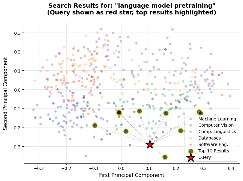
# Visualize search results for a query
query = "language model pretraining"
visualize_search_results(query, embeddings, df, top_k=10)

Top 10 results for query: 'language model pretraining'
================================================================================
1. [0.4240] Reusing Pre-Training Data at Test Time is a Comput...
   Category: cs.CL
2. [0.4102] Evo-1: Lightweight Vision-Language-Action Model wi...
   Category: cs.CV
3. [0.3910] PixCLIP: Achieving Fine-grained Visual Language Un...
   Category: cs.CV
4. [0.3713] PLLuM: A Family of Polish Large Language Models...
   Category: cs.CL
5. [0.3712] SCALE: Upscaled Continual Learning of Large Langua...
   Category: cs.CL
6. [0.3528] Q3R: Quadratic Reweighted Rank Regularizer for Eff...
   Category: cs.LG
7. [0.3334] LLMs and Cultural Values: the Impact of Prompt Lan...
   Category: cs.CL
8. [0.3297] TwIST: Rigging the Lottery in Transformers with In...
   Category: cs.LG
9. [0.3278] IndicSuperTokenizer: An Optimized Tokenizer for In...
   Category: cs.CL
10. [0.3157] Bearing Syntactic Fruit with Stack-Augmented Neura...
   Category: cs.CL

This visualization reveals exactly what's happening during semantic search. The red star represents your query embedding. The black circles highlighted in yellow are the top 10 results. The dotted lines connect the query to its top 10 matches, showing the spatial relationships.

Notice how most of the top results cluster near the query in embedding space. The majority are from the Computational Linguistics category (the green cluster), which makes perfect sense for a query about language model pretraining. Papers from other categories sit farther away in the visualization, corresponding to their lower similarity scores.

You might notice some papers that appear visually closer to the red query star aren't in our top 10 results. This happens because PCA compresses 1536 dimensions down to just 2 for visualization. This lossy compression can't perfectly preserve all distance relationships from the original high-dimensional space. The similarity scores we display are calculated in the full 1536-dimensional embedding space before PCA, which is why they're more accurate than visual proximity in this 2D plot. Think of the visualization as showing general clustering patterns rather than exact rankings.

This spatial representation makes the abstract concept of similarity concrete. High similarity scores mean points that are close together in the original high-dimensional embedding space. When we say two papers are semantically similar, we're saying their embeddings point in similar directions.

Let's try another visualization with a different query:

# Try a more specific query
query = "reinforcement learning algorithms"
visualize_search_results(query, embeddings, df, top_k=10)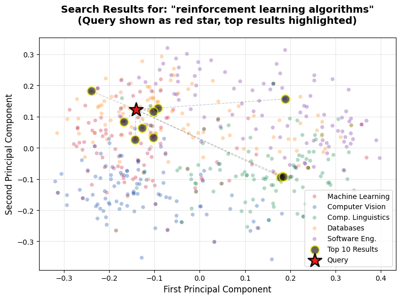

Top 10 results for query: 'reinforcement learning algorithms'
================================================================================
1. [0.3477] Exchange Policy Optimization Algorithm for Semi-In...
   Category: cs.LG
2. [0.3429] Fitting Reinforcement Learning Model to Behavioral...
   Category: cs.LG
3. [0.3091] Online Algorithms for Repeated Optimal Stopping: A...
   Category: cs.LG
4. [0.3062] DeepPAAC: A New Deep Galerkin Method for Principal...
   Category: cs.LG
5. [0.2970] Environment Agnostic Goal-Conditioning, A Study of...
   Category: cs.LG
6. [0.2925] Forgetting is Everywhere...
   Category: cs.LG
7. [0.2865] RLHF: A comprehensive Survey for Cultural, Multimo...
   Category: cs.CL
8. [0.2857] RLHF: A comprehensive Survey for Cultural, Multimo...
   Category: cs.LG
9. [0.2827] End-to-End Reinforcement Learning of Koopman Model...
   Category: cs.LG
10. [0.2813] GrowthHacker: Automated Off-Policy Evaluation Opti...
   Category: cs.SE

This visualization shows clear clustering around the Machine Learning region (red cluster), and most top results are ML papers about reinforcement learning. The query star lands right in the middle of where we'd expect for an RL-focused query, and the top results fan out from there in the embedding space.

Use these visualizations to spot broad trends (like whether your query lands in the right category cluster), not to validate exact rankings. The rankings come from measuring distances in all 1536 dimensions, while the visualization shows only 2.

Evaluating Search Quality

How do we know if our search system is working well? In production systems, you'd use quantitative metrics like Precision@K, Recall@K, or Mean Average Precision (MAP). These metrics require labeled relevance judgments where humans mark which papers are relevant for specific queries.

For this tutorial, we'll use qualitative evaluation. Let's examine results for a query and assess whether they make sense:

# Detailed evaluation of a single query
query = "anomaly detection techniques"
results = semantic_search(query, embeddings, df, top_k=10)

print(f"Query: '{query}'\n")
print(f"Detailed Results:\n{separator}")

for rank, (idx, row) in enumerate(results.iterrows(), 1):
    print(f"\nRank {rank} | Similarity: {row['similarity_score']:.4f}")
    print(f"Title: {row['title']}")
    print(f"Category: {row['category']}")
    print(f"Abstract: {row['abstract'][:200]}...")
    print("-" * 80)

Query: 'anomaly detection techniques'

Detailed Results:
================================================================================

Rank 1 | Similarity: 0.3895
Title: An Encode-then-Decompose Approach to Unsupervised Time Series Anomaly Detection on Contaminated Training Data--Extended Version
Category: cs.DB
Abstract: Time series anomaly detection is important in modern large-scale systems and is applied in a variety of domains to analyze and monitor the operation of
diverse systems. Unsupervised approaches have re...
--------------------------------------------------------------------------------

Rank 2 | Similarity: 0.3268
Title: DeNoise: Learning Robust Graph Representations for Unsupervised Graph-Level Anomaly Detection
Category: cs.LG
Abstract: With the rapid growth of graph-structured data in critical domains,
unsupervised graph-level anomaly detection (UGAD) has become a pivotal task.
UGAD seeks to identify entire graphs that deviate from ...
--------------------------------------------------------------------------------

Rank 3 | Similarity: 0.3218
Title: IEC3D-AD: A 3D Dataset of Industrial Equipment Components for Unsupervised Point Cloud Anomaly Detection
Category: cs.CV
Abstract: 3D anomaly detection (3D-AD) plays a critical role in industrial
manufacturing, particularly in ensuring the reliability and safety of core
equipment components. Although existing 3D datasets like Rea...
--------------------------------------------------------------------------------

Rank 4 | Similarity: 0.3085
Title: Conditional Score Learning for Quickest Change Detection in Markov Transition Kernels
Category: cs.LG
Abstract: We address the problem of quickest change detection in Markov processes with unknown transition kernels. The key idea is to learn the conditional score
$nabla_{\mathbf{y}} \log p(\mathbf{y}|\mathbf{x...
--------------------------------------------------------------------------------

Rank 5 | Similarity: 0.3053
Title: Multiscale Astrocyte Network Calcium Dynamics for Biologically Plausible Intelligence in Anomaly Detection
Category: cs.LG
Abstract: Network anomaly detection systems encounter several challenges with
traditional detectors trained offline. They become susceptible to concept drift
and new threats such as zero-day or polymorphic atta...
--------------------------------------------------------------------------------

Rank 6 | Similarity: 0.2907
Title: I Detect What I Don't Know: Incremental Anomaly Learning with Stochastic Weight Averaging-Gaussian for Oracle-Free Medical Imaging
Category: cs.CV
Abstract: Unknown anomaly detection in medical imaging remains a fundamental challenge due to the scarcity of labeled anomalies and the high cost of expert
supervision. We introduce an unsupervised, oracle-free...
--------------------------------------------------------------------------------

Rank 7 | Similarity: 0.2901
Title: Adaptive Detection of Software Aging under Workload Shift
Category: cs.SE
Abstract: Software aging is a phenomenon that affects long-running systems, leading to progressive performance degradation and increasing the risk of failures. To
mitigate this problem, this work proposes an ad...
--------------------------------------------------------------------------------

Rank 8 | Similarity: 0.2763
Title: The Impact of Data Compression in Real-Time and Historical Data Acquisition Systems on the Accuracy of Analytical Solutions
Category: cs.DB
Abstract: In industrial and IoT environments, massive amounts of real-time and
historical process data are continuously generated and archived. With sensors
and devices capturing every operational detail, the v...
--------------------------------------------------------------------------------

Rank 9 | Similarity: 0.2570
Title: A Large Scale Study of AI-based Binary Function Similarity Detection Techniques for Security Researchers and Practitioners
Category: cs.SE
Abstract: Binary Function Similarity Detection (BFSD) is a foundational technique in software security, underpinning a wide range of applications including
vulnerability detection, malware analysis. Recent adva...
--------------------------------------------------------------------------------

Rank 10 | Similarity: 0.2418
Title: Fraud-Proof Revenue Division on Subscription Platforms
Category: cs.LG
Abstract: We study a model of subscription-based platforms where users pay a fixed fee for unlimited access to content, and creators receive a share of the revenue. Existing approaches to detecting fraud predom...
--------------------------------------------------------------------------------

Looking at these results, we can assess quality by asking:

• Are the results relevant to the query? Yes! All papers discuss anomaly detection techniques and methods.
• Are similarity scores meaningful? Yes! Higher-ranked papers are more directly relevant to the query.
• Does the ranking make sense? Yes! The top result is specifically about time series anomaly detection, which directly matches our query.

Let's look at what similarity score thresholds might indicate:

# Analyze the distribution of similarity scores
query = "query optimization algorithms"
results = semantic_search(query, embeddings, df, top_k=50)

print(f"Query: '{query}'")
print(f"\nSimilarity score distribution for top 50 results:")
print(f"  Highest score: {results['similarity_score'].max():.4f}")
print(f"  Median score: {results['similarity_score'].median():.4f}")
print(f"  Lowest score: {results['similarity_score'].min():.4f}")

# Show how scores change with rank
print(f"\nScore decay by rank:")
for rank in [1, 5, 10, 20, 30, 40, 50]:
    score = results['similarity_score'].iloc[rank-1]
    print(f"  Rank {rank:2d}: {score:.4f}")

Query: 'query optimization algorithms'

Similarity score distribution for top 50 results:
  Highest score: 0.4206
  Median score: 0.2765
  Lowest score: 0.2402

Score decay by rank:
  Rank  1: 0.4206
  Rank  5: 0.3666
  Rank 10: 0.3144
  Rank 20: 0.2910
  Rank 30: 0.2737
  Rank 40: 0.2598
  Rank 50: 0.2402

Similarity score interpretation depends heavily on your dataset characteristics. Here are general heuristics, but they require adjustment based on your specific data:

For broad, multi-domain datasets (like ours with 5 distinct categories):

• 0.40+: Highly relevant
• 0.30-0.40: Very relevant
• 0.25-0.30: Moderately relevant
• Below 0.25: Questionable relevance

For narrow, specialized datasets (single domain):

• 0.70+: Highly relevant
• 0.60-0.70: Very relevant
• 0.50-0.60: Moderately relevant
• Below 0.50: Questionable relevance

The key is understanding relative rankings within your dataset rather than treating these as universal thresholds. Our multi-domain dataset naturally produces lower absolute scores than a specialized single-topic dataset would. What matters is that the top results are genuinely more relevant than lower-ranked results.

Testing Edge Cases

A good search system should handle different types of queries gracefully. Let's test some edge cases:

# Test 1: Very specific technical query
print(f"Test 1: Highly Specific Query\n{separator}")
query = "graph neural networks for molecular property prediction"
results = semantic_search(query, embeddings, df, top_k=3)
print(f"Query: '{query}'\n")
for idx, row in results.iterrows():
    print(f"  [{row['similarity_score']:.4f}] {row['title'][:50]}...")

# Test 2: Broad general query
print(f"\n\nTest 2: Broad General Query\n{separator}")
query = "artificial intelligence"
results = semantic_search(query, embeddings, df, top_k=3)
print(f"Query: '{query}'\n")
for idx, row in results.iterrows():
    print(f"  [{row['similarity_score']:.4f}] {row['title'][:50]}...")

# Test 3: Query with common words
print(f"\n\nTest 3: Common Words Query\n{separator}")
query = "learning from data"
results = semantic_search(query, embeddings, df, top_k=3)
print(f"Query: '{query}'\n")
for idx, row in results.iterrows():
    print(f"  [{row['similarity_score']:.4f}] {row['title'][:50]}...")

Test 1: Highly Specific Query
================================================================================
Query: 'graph neural networks for molecular property prediction'

  [0.3602] ScaleDL: Towards Scalable and Efficient Runtime Pr...
  [0.3072] RELATE: A Schema-Agnostic Perceiver Encoder for Mu...
  [0.3032] Dark Energy Survey Year 3 results: Simulation-base...

Test 2: Broad General Query
================================================================================
Query: 'artificial intelligence'

  [0.3202] Lessons Learned from the Use of Generative AI in E...
  [0.3137] AI for Distributed Systems Design: Scalable Cloud ...
  [0.3096] SmartMLOps Studio: Design of an LLM-Integrated IDE...

Test 3: Common Words Query
================================================================================
Query: 'learning from data'

  [0.2912] PrivacyCD: Hierarchical Unlearning for Protecting ...
  [0.2879] Learned Static Function Data Structures...
  [0.2732] REMIND: Input Loss Landscapes Reveal Residual Memo...

Notice what happens:

• Specific queries return focused, relevant results with higher similarity scores
• Broad queries return more general papers about AI with moderate scores
• Common word queries still find relevant content because embeddings understand context

This demonstrates the power of semantic search over keyword matching. A keyword search for "learning from data" would match almost everything, but semantic search understands the intent and returns papers about data-driven learning and optimization.

Understanding Retrieval Quality

Let's create a function to help us understand why certain papers are retrieved for a query:

def explain_search_result(query, paper_idx, embeddings, df):
    """
    Explain why a particular paper was retrieved for a query.
    """
    # Get query embedding
    response = co.embed(
        texts=[query],
        model='embed-v4.0',
        input_type='search_query',
        embedding_types=['float']
    )
    query_embedding = np.array(response.embeddings.float_[0])

    # Calculate similarity
    paper_embedding = embeddings[paper_idx]
    similarity = cosine_similarity(
        query_embedding.reshape(1, -1),
        paper_embedding.reshape(1, -1)
    )[0][0]

    # Show the result
    print(f"Query: '{query}'")
    print(f"\nPaper: {df['title'].iloc[paper_idx]}")
    print(f"Category: {df['category'].iloc[paper_idx]}")
    print(f"Similarity Score: {similarity:.4f}")
    print(f"\nAbstract:")
    print(df['abstract'].iloc[paper_idx][:300] + "...")

    # Show how this compares to all papers
    all_similarities = cosine_similarity(
        query_embedding.reshape(1, -1),
        embeddings
    )[0]
    rank = (all_similarities > similarity).sum() + 1

    print(f"\nRanking: {rank}/{len(df)} papers")
    percentage = (len(df) - rank)/len(df)*100
    print(f"This paper is more relevant than {percentage:.1f}% of papers")

# Explain why a specific paper was retrieved
query = "database query optimization"
paper_idx = 322
explain_search_result(query, paper_idx, embeddings, df)

Query: 'database query optimization'

Paper: L2T-Tune:LLM-Guided Hybrid Database Tuning with LHS and TD3
Category: cs.DB
Similarity Score: 0.3374

Abstract:
Configuration tuning is critical for database performance. Although recent
advancements in database tuning have shown promising results in throughput and
latency improvement, challenges remain. First, the vast knob space makes direct
optimization unstable and slow to converge. Second, reinforcement ...

Ranking: 9/500 papers
This paper is more relevant than 98.2% of papers

This explanation shows exactly why the paper was retrieved: it has a solid similarity score (0.3373) and ranks in the top 2% of all papers for this query. The abstract clearly discusses database configuration tuning and optimization, which matches the query intent perfectly.

Applying These Skills to Your Own Projects

You now have a complete semantic search system. The skills you've learned here transfer directly to any domain where you need to find relevant documents based on meaning.

The pattern is always the same:

1. Collect documents (APIs, databases, file systems)
2. Generate embeddings (local models or API services)
3. Store embeddings efficiently (files or vector databases)
4. Implement similarity calculations (cosine, dot product, or Euclidean)
5. Build a search function that returns ranked results
6. Evaluate results to ensure quality

This exact workflow applies whether you're building:

• A research paper search engine (what we just built)
• A code search system for documentation
• A customer support knowledge base
• A product recommendation system
• A legal document retrieval system

For the upcoming practice project, you'll apply these techniques to build a Kaggle dataset search engine. The process is identical:

1. Use the Kaggle API to collect data
2. Generate embeddings for dataset descriptions
3. Implement similarity calculations
4. Build a search function
5. Evaluate results

The only difference is the data source. Everything else remains the same.

Optimizing for Production

Before we wrap up, let's discuss a few optimizations for production systems. We won't implement these now, but knowing they exist will help you scale your search system when needed.

1. Caching Query Embeddings

If users frequently search for similar queries, caching the embeddings can save significant API calls and computation time. Store the query text and its embedding in memory or a database. When a user searches, check if you've already generated an embedding for that exact query. This simple optimization can reduce costs and improve response times, especially for popular searches.

2. Approximate Nearest Neighbors

For datasets with millions of embeddings, exact similarity calculations become slow. Libraries like FAISS, Annoy, or ScaNN provide approximate nearest neighbor search that's much faster. These specialized libraries use clever indexing techniques to quickly find embeddings that are close to your query without calculating the exact distance to every single vector in your database. While we didn't implement this in our tutorial series, it's worth knowing that these tools exist for production systems handling large-scale search.

3. Batch Query Processing

When processing multiple queries, batch them together for efficiency. Instead of generating embeddings one query at a time, send multiple queries to your embedding API in a single request. Most embedding APIs support batch processing, which reduces network overhead and can be significantly faster than sequential processing. This approach is particularly valuable when you need to process many queries at once, such as during system evaluation or when handling multiple concurrent users.

4. Vector Database Storage

For production systems, use vector databases (Pinecone, Weaviate, Chroma) rather than files. Vector databases handle indexing, similarity search optimization, and storage efficiency automatically. They also apply float32 precision by default for memory efficiency. Something you'd need to handle manually with file-based storage (converting from float64 to float32 can halve storage requirements with minimal impact on search quality).

5. Document Chunking for Long Content

In our tutorial, we embedded entire paper abstracts as single units. This works fine for abstracts (which are naturally concise), but production systems often process longer documents like full papers, documentation, or articles. Industry best practice is to chunk these into coherent sections (typically 200-1000 tokens per chunk) for optimal semantic fidelity. This ensures each embedding captures a focused concept rather than trying to represent an entire document's diverse topics in a single vector. Modern models with high token limits (8k+ tokens) make this less critical than before, but chunking still improves retrieval quality for longer content.

These optimizations become critical as your system scales, but the core concepts remain the same. Start with the straightforward implementation we've built, then add these optimizations when performance or cost becomes a concern.

What You've Accomplished

You've built a complete semantic search system from the ground up! Let's review what you've learned:

1. You understand three distance metrics (Euclidean distance, dot product, cosine similarity) and when to use each one.
2. You can implement similarity calculations both manually (to understand the math) and efficiently (using scikit-learn).
3. You've built a search function that converts queries to embeddings and returns ranked results.
4. You can visualize search results in embedding space to understand spatial relationships between queries and documents.
5. You can evaluate search quality qualitatively by examining results and similarity scores.
6. You understand how to optimize search systems for production with caching, approximate search, batching, vector databases, and document chunking.

Most importantly, you now have the complete skillset to build your own search engine. You know how to:

• Collect data from APIs
• Generate embeddings
• Calculate semantic similarity
• Build and evaluate search systems

Next Steps

Before moving on, try experimenting with your search system:

Test different query styles:

• Try very short queries ("neural nets") vs detailed queries ("applying deep neural networks to computer vision tasks")
• See how the system handles questions vs keywords
• Test queries that combine multiple topics

Explore the similarity threshold:

• Set a minimum similarity threshold (e.g., 0.30) and see how many results pass
• Test what happens with a very strict threshold (0.40+)
• Find the sweet spot for your use case

Analyze failure cases:

• Find queries where the results aren't great
• Understand why (too broad? too specific? wrong domain?)
• Think about how you'd improve the system

Compare categories:

• Search for "deep learning" and see which categories dominate results
• Try category-specific searches and verify papers match
• Look for interesting cross-category papers

Visualize different queries:

• Create visualizations for queries from different domains
• Observe how the query point moves in embedding space
• Notice which categories cluster near different types of queries

This experimentation will sharpen your intuition about how semantic search works and prepare you to debug issues in your own projects.

---

Key Takeaways:

• Euclidean distance measures straight-line distance between vectors and is the most intuitive metric
• Dot product multiplies corresponding elements and is computationally efficient
• Cosine similarity measures the angle between vectors and is the standard for text embeddings
• For well-normalized embeddings, all three metrics typically produce similar rankings
• Similarity scores depend on dataset characteristics and should be interpreted relative to your specific data
• Multi-domain datasets naturally produce lower absolute scores than specialized single-topic datasets
• Visualizing search results in 2D embedding space helps understand clustering patterns, though exact rankings come from the full high-dimensional space
• The spatial proximity of embeddings directly corresponds to semantic similarity scores
• Production search systems benefit from query caching, approximate nearest neighbors, batch processing, vector databases, and document chunking
• The semantic search pattern (collect, embed, calculate similarity, rank) applies universally across domains
• Qualitative evaluation through manual inspection is crucial for understanding search quality
• Edge cases like very broad or very specific queries test the robustness of your search system
• These skills transfer directly to building search systems in any domain with any type of content