Ok, so I finally got a chance to finish this three-part series. It’s been a long one, but better late than never. Since it’s been a while, I figured a quick recap is in order.

To show how to approach an unguided data project, I decided to use some Netflix data to demonstrate the process across three projects. The first was a fairly basic exploratory analysis of the dataset that used some foundational skills in data wrangling and visualization. Moving on from that was implementing the Shiny package to upgrade some of the visualization by introducing some dynamic elements. All-in-all, the case study shown here isn’t too difficult; it’s just a lot of busy work (aka. real-life data work).

Since I had already looked at the data, the next logical step would be to use this data for some real-life purpose. So, what better way to do so than by creating the classical recommender system, a staple application in machine learning.

What Are Content Based Recommender Systems and Why Are They Useful?

You’re probably familiar with the recommender system, principally because of the rise of YouTube, Amazon and other streaming consumer-based web services. However, if you’re ever in need of a quick definition for this (say in an interview for a data science position), you can explain it as a filter-based application of an algorithm that tries to predict preferences (i.e., movies, songs, video clips, products) in accordance with some known factors.

Generally speaking, there are a few major types of recommender systems in use. One type is the collaborative-based model. As the name suggests, it uses the input of multiple past users to produce recommendations for future users. Usually, it’ll be a historic rating profile.

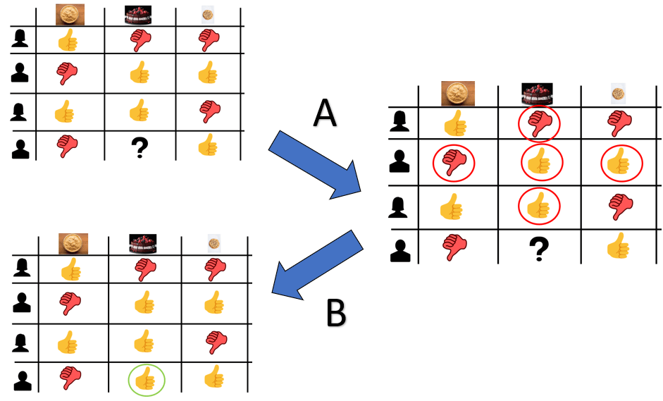
Figure 1. In this case, the rating history of past members for cakes/pies/cookies as dessert will help predict whether or not to recommend cake as a dessert in relation to said person’s opinions about pies and cookies.

While this method has the benefit of not needing domain knowledge to determine recommendations, it does have a few drawbacks:

1. Cold start: an issue where a system or a part of a system isn’t working normally due to the lack of connection being made prior to using the model. In other words, if there isn’t anything to go off of initially, it’s a wild guess as to whether or not the recommendation will be any better than just randomly picking something.
2. Sparsity: considering that there is a vast amount of content/inventory that can potentially exist, it is possible that the majority of ratings are only for a small subset of items, and this leaves little to go on for potentially valuable choices.
3. Scalability: with millions of users and/or content possible in a database, a lot of computational power would be necessary.

While this would have been a perfectly valid option, this Netflix data doesn’t have any sort of data pertaining to user behavior, and it only consists of info pertaining to the content. Thus, we will have to use an alternative model known as the content-based recommender system. As the name suggests, it’s a method that relies on the description profile of the item to generate recommendations.

This is something that happens when you go to a store and ask a salesperson to recommend a product (say, a car) based on some of your important purchasing qualities. However, you really just automate this process by filling out some kind of user profile.

Figure 2. It's sort of like going to a car dealership to grab some options, but without the useless undercoat upsell.

While this method does have its flaws with respect to scalability and its limitation in recommending anything outside of your original preference setting, it does solve the “cold start” or “sparsity” issue because it doesn’t rely on existing connections to make predictions. It is just based on the weight of each feature, which denotes the importance to the user.

So that’s enough about the theory of the recommender system. Let’s move onto how to make it happen using our Netflix dataset.

The Plan

Like all things, we’ll start with a quick visual of how I would like this project to look. In my mind, it should look like this:

Figure 3. So clearly, we'll need to use the Shiny package here.

In terms of the backend side of things, you can choose many algorithms to facilitate recommendations. This is the first of many factors that determine the quality of your recommender system. Considering the system’s simplicity and its ability to produce fairly competitive results with more complex algorithms, we’ll be using two approaches: (1) clustering and (2) K-Nearest Neighbor (KNN) modelling to generate our recommendations.

Now that we’ve determined the recommender system type and method, the next important factor is how to assess the data to generate those recommendations. Typically, options like Euclidean or Manhattan’s distance work for most cases (as in KNN modelling). However, some consideration is important here because certain distance metrics work better for particular data types. Considering that this dataset contains predominantly qualitative data with a great deal of dimensionality, we’ll use an alternative to the typical distance metric in the form of (1) Jaccard’s distance for the KNN approach and (2) Gower’s distance, measures dissimilarity between individuals for the clustering. (The details of this metric are beyond the scope of this post, but you can read them here, here, and here.) However, the TLDR rationale for choosing this is that it allows us to measure distance between non-numerical data.

Now unlike the KNN approach, the clustering approach will use three different content inputs instead of just one because we would like to specifically understand one’s interest profile in streaming content to generate recommendations. However, these inputs will differ based on the individual’s ranking of the three types of content, which means we will introduce a weighting factor in the algorithm. This weighting factor should be both large enough to demonstrate difference between the choices as well as small enough to not drastically affect the recommendations provided.

Now that we know the general process, the last thing we’ll need to determine is which of the available variables we should use in our clustering approach. Normally, you would do some in-depth market research with a subsample of the target population to identify trends or patterns between content and watchability (likely measured in terms of a rating system or viewing frequency). Since it’s clear that we don’t have that knowledge at hand, nor the resources to even try to find that answer, the next best thing would be to use your best judgment in selecting variables that would affect watchability. After some initial exploration and some reasonable assumptions, we’ll use the following variables from the dataset:

• Show ID — we need this for the recommender system to work
• Content type — some people prefer watching TV series over movies, and vice versa
• Title — we need this for the recommender system to work
• Cast — this assumes that the actors in the content can affect popularity/watchability
• Listed in — contains a list of genres (three, max.)
• Country — used to differentiate English and non-English content
• Rating — the content rating (e.g., PG-13 or TV-MA)
• Description — we need this for the end product
• Release Year — determines the age of the content

Because the cast can be large, we’ll consider the headlining cast member (i.e., the lead actor or actress) as the most important influence on viewership. So, we’ll only include those actors or actresses.

Now, let’s work through the plan step-by-step.

The Process

As with any data project, we begin with some pre-processing of the Netflix dataset. With both approaches to generating recommendations, the initial process will be the same. We need to accomplish the following:

1. Create a DataFrame of only the lead director and headlining actor/actress after extracting them from the listed cast members.

   ```
   # Subset the data to only get the lead cast member 
   netflix_lead = as.data.frame(str_split(netflix$cast, ",", simplify = TRUE)[, 1]) 
   colnames(netflix_lead) = "cast_lead"

2. Differentiate Netflix content based on whether it is presumably English-speaking content or not based on listed genre, country of origin, and title.
<pre><code class="language-r">```
# Create a means to differentiate content as either English-speaking or not based on genre 
library(tidyverse)
netflix_english_content = netflix
                            mutate(
                              non_english_content = 
                                     ifelse(str_detect(listed_in, "(.+/s)?British TV Shows(.+/s)?") == TRUE, FALSE,
                                     ifelse(str_detect(listed_in, "(.+/s)?International TV Shows(.+/s)?|(.+/s)?International Movies(.+/s)?|(.+/s)?Anime Series(.+/s)?|(.+/s)?Anime Features(.+/s)?|(.+/s)?Korean TV Shows(.+/s)?|(.+/s)?Spanish-Language TV Shows(.+/s)?") == TRUE, TRUE, FALSE))
                              )

# Create a means for differentiating content as English-speaking based on country of origin
netflix_english_nation = netflix
                            mutate(
                              in_english_nation = ifelse(str_detect(country, "(.+/s)?United States(.+/s)?|(.+/s)?United Kingdom(.+/s)?|(.+/s)?Canada(.+/s)?|(.+/s)?Australia(.+/s)?|(.+/s)?New Zealand(.+/s)?|(.+/s)?Ireland(.+/s)?|(.+/s)?Jamaica(.+/s)?|(.+/s)?Barbados(.+/s)?") == TRUE, TRUE, FALSE)
                              )

# Create a function that looks at characters in the title to see if it meets a cut-off criterion 
is_not_english = function(string){
  some_count = 0 # Give a running count for any instance of non-ASCII character 

  for(char in str_split(string, boundary("character"))[[1]]){
    if(str_detect(char, "[A-Za-z0-9 \\*\\!\\(\\):,&\\@\\'
      some_count = some_count + 1
    }
  }
  # Characters with at least 2 non-ASCII character = likely not English
  outcome = ifelse(some_count >= 2, "Likely Not English", "Likely English") 

  return(outcome)
}

# Apply function to propose whether the content is English-speaking or not based on title 
netflix_cleaning = cbind(as.data.frame(unlist(map(netflix$title, is_not_english)))
                                    rename(is_english = "unlist(map(netflix$title, is_not_english))"), netflix)

# Determine content as either English-speaking or not based on a consensus of these three variables and then combine with the original Netflix data set into one
english_check = cbind(netflix_english_nation

final_english_check = english_check
  select(title ,non_english_content, is_english, in_english_nation, cast, director, description)
  mutate( assume_english = 
        ifelse(c(non_english_content == T & in_english_nation == T & is_english == "Likely English"), "no",
        ifelse(c(non_english_content == T & in_english_nation == F & is_english == "Likely English"), "no",              
        ifelse(c(non_english_content == T & in_english_nation == T & is_english == "Likely Not English"), "no",
        ifelse(c(non_english_content == T & in_english_nation == F & is_english == "Likely Not English"), "no", 
        ifelse(c(non_english_content == F & in_english_nation == T & is_english == "Likely English"), "yes",
        ifelse(c(non_english_content == F & in_english_nation == F & is_english == "Likely English"), "no",
        ifelse(c(non_english_content == F & in_english_nation == T & is_english == "Likely Not English"), "no", "no")))))))
  )

english_check = as.data.frame(final_english_check$assume_english)

netflix_english = cbind(netflix, english_check) 

netflix_english = netflix_english

```

# Transform the newly formed variables into the appropriate data type
netflix_combine = netflix_combine mutate(
is_english = ifelse(is_english == "no", 0, 1),
cast_lead = ifelse(is.na(cast_lead), "Unknown/No Lead", cast_lead)
) mutate(
cast_lead = as.factor(cast_lead)
)
```
With the dataset now prepped, the next step would be to create dummy variables with the categorical variables in the dataset, which includes each listed director and cast member using the dummy_cols() function from the fastDummies package.

<em>Note: with 7,787 entries and multiple dimensions with a given variable, this will take a while to run or fail due to the number of options. This explains the difficulty in scaling a content-based recommender system.</em>
<pre><code class="language-r">```
# “Dummify” the categorical variable
netflix_combine_for_knn = fastDummies::dummy_cols(netflix_combine, select_columns = c("cast_lead"), remove_selected_columns = TRUE)
```
The next step would be to create a matrix containing all of the relevant entries that would be used in our algorithms (i.e., everything minus the title of the content, description of content, whether the content is a movie/TV show). This is where the processes of the two machine learning algorithms begin to differ. When using a KNN model, we need to calculate the Jaccard’s distance, which is possible with the dist() function with the input as method = “binary”.
<pre><code class="language-r">```
netflix_for_matrix = netflix_combine_for_knn rownames(netflix_for_matrix) = netflix_for_matrix[, 1] # Using show id for both column and row names in the matrix
netflix_for_matrix = netflix_for_matrix netflix_matrix = as.matrix(dist(netflix_for_matrix, method = "binary")) # FOR KNN APPROACH

```
<img loading="lazy" src="https://www.dataquest.io/wp-content/uploads/2022/01/building-recommender-system-table1.jpg.webp" alt="Matrix with Relevant Entries" width="1499" height="462" class="aligncenter wp-image-37084 size-full" srcset="https://www.dataquest.io/wp-content/uploads/2022/01/building-recommender-system-table1.jpg.webp 1499w, https://www.dataquest.io/wp-content/uploads/2022/01/building-recommender-system-table1.jpg-340x105.webp 340w, https://www.dataquest.io/wp-content/uploads/2022/01/building-recommender-system-table1.jpg-1024x316.webp 1024w, https://www.dataquest.io/wp-content/uploads/2022/01/building-recommender-system-table1.jpg-768x237.webp 768w" sizes="(max-width: 1499px) 100vw, 1499px" />

<a href="https://www.dataquest.io/wp-content/uploads/2022/01/building-recommender-system-table2.jpg.webp"><img loading="lazy" src="https://www.dataquest.io/wp-content/uploads/2022/01/building-recommender-system-table2.jpg.webp" alt="Recommender System Chart" width="1346" height="527" class="size-full wp-image-37085 aligncenter" srcset="https://www.dataquest.io/wp-content/uploads/2022/01/building-recommender-system-table2.jpg.webp 1346w, https://www.dataquest.io/wp-content/uploads/2022/01/building-recommender-system-table2.jpg-340x133.webp 340w, https://www.dataquest.io/wp-content/uploads/2022/01/building-recommender-system-table2.jpg-1024x401.webp 1024w, https://www.dataquest.io/wp-content/uploads/2022/01/building-recommender-system-table2.jpg-768x301.webp 768w" sizes="(max-width: 1346px) 100vw, 1346px" /></a>

When using the clustering approach with Gower’s distance as the metric, we need to use the <a href="https://www.rdocumentation.org/packages/cluster/versions/2.1.2/topics/daisy" target="_blank" rel="noopener">daisy()</a> function from the cluster pack
<pre><code class="language-r">```
dissimilarity_gower_1 = as.matrix(daisy(netflix_gower_combine_1, metric = "gower"))
row.names(dissimilarity_gower_1) = netflix_gower_combine$show_id
colnames(dissimilarity_gower_1) = netflix_gower_combine$show_id

```
<a href="https://www.dataquest.io/wp-content/uploads/2022/01/building-recommender-system-table3.jpg-min-_1_.webp"><img loading="lazy" src="https://www.dataquest.io/wp-content/uploads/2022/01/building-recommender-system-table3.jpg-min-_1_.webp" alt="" width="960" height="460" class="size-full wp-image-37087 aligncenter" srcset="https://www.dataquest.io/wp-content/uploads/2022/01/building-recommender-system-table3.jpg-min-_1_.webp 960w, https://www.dataquest.io/wp-content/uploads/2022/01/building-recommender-system-table3.jpg-min-_1_-340x163.webp 340w, https://www.dataquest.io/wp-content/uploads/2022/01/building-recommender-system-table3.jpg-min-_1_-768x368.webp 768w" sizes="(max-width: 960px) 100vw, 960px" /></a>

<a href="https://www.dataquest.io/wp-content/uploads/2022/01/building-recommender-system-table4.jpg-min.webp"><img loading="lazy" src="https://www.dataquest.io/wp-content/uploads/2022/01/building-recommender-system-table4.jpg-min.webp" alt="" width="954" height="317" class="size-full wp-image-37088 aligncenter" srcset="https://www.dataquest.io/wp-content/uploads/2022/01/building-recommender-system-table4.jpg-min.webp 954w, https://www.dataquest.io/wp-content/uploads/2022/01/building-recommender-system-table4.jpg-min-340x113.webp 340w, https://www.dataquest.io/wp-content/uploads/2022/01/building-recommender-system-table4.jpg-min-768x255.webp 768w" sizes="(max-width: 954px) 100vw, 954px" /></a>

The last step is to create a function to generate recommendations. Using the KNN approach, this will involve (1) creating a vector to store the findings, (2) running through each entry in the dataset to skip over any exact title matches of the input, and (3) gathering the top matching content based on the K-number selected. In this case, the shorter the distance metric corresponds to a greater presumed match to the input.
<pre><code class="language-r">```
new_recommendation = function(title, data, matrix, k, reference_data){

# translate the title to show_id

show_id = reference_data$show_id[reference_data$title == title]

# create a holder vector to store findings
id = rep(0, nrow(data))
metric = rep(0, nrow(data))
content_title = reference_data$title
description = reference_data$description
country = reference_data$country
genres = reference_data$listed_in
type = reference_data$type

for(i in 1:nrow(data)) {
if(rownames(data)[i] == show_id) {
next # used to skip any exact titles used from the input
}
id[i] = colnames(matrix)[i]
metric[i] = matrix[show_id, i]
}

choices = cbind(as.data.frame(id), as.data.frame(content_title), as.data.frame(description), as.data.frame(metric), as.data.frame(type), as.data.frame(country), as.data.frame(genres))
choices = choices choices = as.data.frame(choices)
return(choices[0:(k+1),])
}

View(new_recommendation(“The Other Guys”, netflix_for_matrix, netflix_matrix, 15, netflix))
```
<img loading="lazy" src="https://www.dataquest.io/wp-content/uploads/2022/01/building-recommender-system-table5.jpg.webp" alt="" width="991" height="377" class="size-full wp-image-37089 aligncenter" srcset="https://www.dataquest.io/wp-content/uploads/2022/01/building-recommender-system-table5.jpg.webp 991w, https://www.dataquest.io/wp-content/uploads/2022/01/building-recommender-system-table5.jpg-340x129.webp 340w, https://www.dataquest.io/wp-content/uploads/2022/01/building-recommender-system-table5.jpg-768x292.webp 768w" sizes="(max-width: 991px) 100vw, 991px" />
<p class="text-center"><em>Figure 4. Looking at the recommendations provided, it doesn’t seem to be too shabby for an action comedy like the “The Other Guys” with Will Farrell and Mark Wahlberg.</em></p>
When using Gower’s distance, the approach would be slightly different because we’ll be converting a dissimilarity matrix into a DataFrame. In this case, it’ll involve (1) filtering the matrix to only include columns corresponding to the content input that we would like to find recommendations for using the which() function, (2) reorganizing the DataFrame to list all the dissimilarity scores on a single column via the pivot_longer() function, (3) removing exact matches to the input content from the recommendation pool, (4) creating a metric that measures similarity of titles, which would be 1-dissimilarity score (i.e., Gower’s distance), and (5) grouping and arranging the data in accordance to the similarity score.

Unlike the previous method, the three Netflix content inputs for which recommendations would be generated should have an effect. In this case, the most “favorited” one would have a greater impact than the least favorited one, which means that there should be a weighted factor. The key to this is to select the right weighted value that’s not so large that it skews your recommendations to your top pick but large enough that we can observe these differences in the recommendations. This process is much more of an art than a science, particularly in the absence of an actually conducted study. However, through trial and error, a weighted factor of 1.1 applied to the top favorited choice, 1.05 for the second favorited choice, and 1 for the third choice would be the best approach.

So, with that determined, let’s show how this algorithm works. Using Sense8, Adam Ruins Everything, and The Waterboy as the proposed favorite, secondary and tertiary choices, the generation of recommended titles using a reconverted dissimilarity matrix would look like this:
<pre><code class="language-r">```
test_selection = netflix_gower_combine test_selection = test_selection

select_data_indices = which(colnames(dissimilarity_gower_1)

test_selection_result_data = data.frame(
dissimilarity_gower_1[, select_data_indices],
recommended_netflix_content = row.names(dissimilarity_gower_1)
)

something_here_1 = test_selection_result_data pivot_longer(
cols = c(-"recommended_netflix_content"),
names_to = "watched_content",
values_to = "dissimilarity_gower_1"
) left_join(test_selection, by = c("watched_content" = "show_id")) filter(recommended_netflix_content != watched_content) mutate(
similarity = 1-dissimilarity_gower_1,
weighted_similarity = similarity*ranking
) group_by(recommended_netflix_content) arrange(desc(weighted_similarity)) slice(1) arrange(desc(weighted_similarity))

top_recommendations_1 = something_here_1

top_recommendations_1 = top_recommendations_1 left_join(netflix_gower_combine, by = c("recommended_netflix_content" = "show_id")) select(recommended_netflix_content, title.y, description.y, weighted_similarity, type.y, cast_lead.y)

top_recommendations_1

recommendations = top_recommendations_1$title.y
```

Figure 5. The recommendations could be better here.

Boom! We’ve got a working Netflix content-based recommender system using two different algorithms here. Pretty sweet right? Obviously, we can automate this by including each of the above steps into a singular function. (You can check out that code

Figure 7. Using Jaccard's distance to determine Netflix recommendations

There we have it. We’ve got a fully functioning Shiny web app that provides a number of TV series/movie recommendations based on some of your favorites. Pretty cool, huh? If you want to see how this is coded, you can There we have it. We finally reached the end of this series, putting into action some of the advice I mentioned earlier. Thanks for following along, and I hope that you found some knowledge and/or inspiration to help you with your own unguided projects.

If you’re interested in checking out some of my other projects, you can head over to my GitHub. Alternatively, if you’re got some idea on a collaborative project or just want to connect, hit me up on my LinkedIn.

Happy projecting all!